This started with a fairly simple question#
“Can we get at least 1.3×?”
That was the goal. There was a competition called the Open Kernel Challenge, people were posting speedups over an existing implementation, and I wanted to see how far I could get.
The first version I tested came back at 0.7761×.
If you're wondering whether that's good: no. One means I matched the starting point. Below one means I made it slower. The code gave the right answers, but it took longer to get them.
So this became a story about figuring out what “faster” actually requires. Sometimes I needed more work running at once. Sometimes I needed to move the same numbers into a different arrangement. Sometimes the best move was to keep using an existing library. And quite a few things that sounded clever just lost.
I eventually got an official 1.30×, then 1.3234×, on the part of the model I was working on. I'll explain what that means in a bit. It doesn't mean the entire AI model suddenly got 32% faster.
I worked with Claude and Codex along the way. This is my walkthrough of that process: what I tried, what the results said, and what I kept. I'm going to build the math and the GPU concepts from the ground up, then use them to explain the real experiments. No linear algebra or CUDA background assumed. The point is to understand the work well enough that the next design choice makes sense.
This is a long read. I use small numerical examples first, then connect them to the actual source and timings. When I say an example is illustrative, its numbers explain a concept; the experiment tables are the recorded results. You can leave and come back using the section links below the title.
Okay, what is the model doing in the first place?#
When you send a message to a language model, it turns the text into tokens. A token is a small piece of text: sometimes a word, sometimes part of a word, sometimes punctuation. The model represents those tokens as lists of numbers and runs calculations on them to predict what should come next.
A lot of those calculations are variations of the same thing: take some input numbers, multiply them by some stored numbers, and add the results.
Those stored numbers are called weights. Training chooses the weights. When I'm running the model to answer a message, the weights are already there; I'm using them to transform the input. That answering stage is called inference.
Here's a deliberately tiny example. Say the input is [2, 3], and one set of weights is [4, -1]. Multiply matching entries, then add them:
A different set of weights, [1, 2], gives 2 × 1 + 3 × 2 = 8. So the same input can produce an output list [5, 8]. A dense projection does this sort of weighted sum over much bigger lists. “Dense” means the calculation uses the full matrix of weights rather than a selected sparse subset.
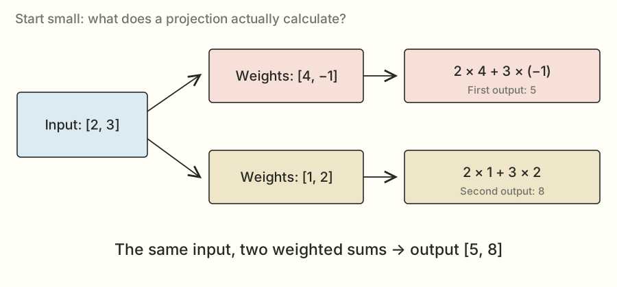
Put lots of input lists and weight lists into rectangular tables, and you get matrix multiplication. The tables are matrices. The multiplication is a compact way to ask for all those weighted sums.
The real calculation might use 8,192 input numbers for each token and produce thousands of outputs. Repeat this inside a model, over many tokens, and small differences in how you run the calculation start to matter.
I'm going to unpack the math properly#
The little weighted-sum example is the calculation I kept coming back to. But I want to build the vocabulary around it carefully, because later choices about tiles, reductions, and transposes make much more sense when the math is familiar.
Start with a scalar: one number, like 3. A vector is an ordered list of numbers, like [2, 3]. A matrix is a rectangular arrangement of numbers, like a spreadsheet with a fixed number of rows and columns. A tensor is the more general term for an array with some number of dimensions. A scalar, vector, and matrix can be viewed as zero-, one-, and two-dimensional tensors.
Here, “dimension” can mean two related things. The vector [2, 3] has two coordinates. A matrix has two axes, rows and columns, but each of those axes can contain thousands of entries. When I say the matrix has shape [16, 8,192], I'm saying it has 16 rows and 8,192 columns. I'm not saying it has only two stored numbers.
The order matters. [2, 3] and [3, 2] are different vectors. Swapping input features while leaving their weights alone generally changes the answer, just as swapping the quantity and price columns in a spreadsheet would change what a formula means.
Addition and scaling come first#
To add two vectors of the same length, add matching entries. [2, 3] + [1, -2] = [3, 1]. To multiply a vector by a scalar, multiply every entry: 4 × [2, 3] = [8, 12].
Those operations already explain part of what a projection does. A weight scales how much one input feature contributes to an output. A positive weight contributes in the same sign as the input; a negative weight can subtract. A zero weight contributes nothing to that particular sum.
I don't need to attach a human-readable meaning like “happiness” or “grammar” to each feature. Inside a learned model, the coordinates are learned numerical representations. My kernel's job is to transform the numbers according to the specified weights, regardless of what an individual coordinate might mean.
A dot product makes one output number#
The dot product of two equally long vectors multiplies corresponding entries and adds the products:
The result is one scalar. It isn't the vector [8, -3]; that vector would be the elementwise product before the final addition. This distinction will matter in the expert block later, where some multiplications really are element by element.
For a longer example, take [1, -2, 3] and [4, 5, -1]. Their products are 4, -10, and -3. Add them and the dot product is -9. Negative answers are perfectly ordinary. A linear projection is not a probability calculation by itself.
If you've seen the symbol Σ and wondered where the complicated math started, this is all it is doing here: telling me to add a sequence of terms. I can write the same dot product as Σₖ xₖwₖ. The little k is an index pointing to matching positions in the two lists.
In code I usually start indices at zero. With K input features, the positions are 0, 1, …, K−1. That gives K positions, just as the floors numbered 0 through 4 give five floors.
Matrix multiplication is a whole collection of dot products#
I'll keep two token rows together in an input matrix X, and use three weight rows in W:
 2   3
 1  −2
 4  −1
 1   2
−2   3
For the first token row [2, 3], I take a dot product with every row of W. They give 5, 8, and 5. For the second token row [1, -2], the same three weight rows give 6, -3, and -8.
The output matrix is therefore:
There are six output cells because there are two tokens and three output features: 2 × 3 = 6. Every output is a dot product of length two, because every input row and every weight row have two features.
Try selecting an output cell below. The highlighted input row and weight row are the two vectors used for that cell. Move the slider to include zero, one, or both terms of the sum.
Teaching example · exact small integers · no benchmark claims
X
| 2 | 3 |
| 1 | -2 |
W
| 4 | -1 |
| 1 | 2 |
| -2 | 3 |
Wᵀ
| 4 | 1 | -2 |
| -1 | 2 | 3 |
Y
| 5 | 8 | 5 |
| 6 | -3 | -8 |
X row 0 meets W row 0, which becomes column 0 of Wᵀ.
The bottom-right output is a useful one to check by hand. Its input is [1, -2]; its weights are [-2, 3]. So it is 1 × (-2) + (-2) × 3 = -2 - 6 = -8. If you can follow that calculation, you can follow the mathematical operation inside the real projection. The GPU version makes the arrays bigger and the execution much more organized.
Why the transpose appears#
The standard rule for matrix multiplication says: a row of the left matrix meets a column of the right matrix. I stored each output's weights in a row of W, so I use W's transpose to make those rows appear as columns.
For this example:
 4  −1
 1   2
−2   3
 4   1  −2
−1   2   3
Transposing changes which axis I call rows and which I call columns. It doesn't turn 4 into some new numerical value. Later I'll distinguish viewing an array with different strides from actually copying it into a new contiguous order. Both can describe the same logical transpose while creating different memory-access behavior.
Now the shapes line up:
[2, 2] × [2, 3] → [2, 3]
The inner dimensions match because each dot product needs two equally long vectors. The outer dimensions remain because I need one result for every input row and every output feature.
This also explains why matrix multiplication usually can't be swapped around. Changing A × B to B × A changes which rows meet which columns, and sometimes the dimensions don't even permit the swapped product. A library-layout experiment needs an algebraically equivalent transformation, not a casual reordering of the multiplication.
The full equation, now with the letters explained#
For this task, the output cell at token row m and output feature n is:
Read it slowly: choose one token row m; choose one output n; visit every input feature k; multiply the input by the matching weight; add those products. That's it. M counts how many token rows I have, N counts how many outputs each needs, and K counts how long each sum is.
Here's the straightforward loop version. It's for understanding the math, not the implementation I submitted:
for m in range(M):
    for n in range(N):
        total = 0
        for k in range(K):
            total += X[m, k] * W[n, k]
        Y[m, n] = total
The output cells can be computed independently in exact arithmetic. But the K terms within one cell have to be combined. That difference between independent output work and a reduction into one answer is the reason split-K will show up in the experiment story.
What makes it linear?#
A transformation T is linear when it preserves addition and scalar multiplication: T(a + b) = T(a) + T(b) and T(ca) = cT(a). A fixed matrix multiplication has those properties in exact arithmetic. For example, using the weight row [4, -1], the inputs [2, 3] and [1, -2] produce 5 and 6. Add the inputs to get [3, 1], and the output is 12 - 1 = 11, which is also 5 + 6.
That doesn't make the entire language model linear. The model also contains nonlinear functions, normalizations, attention probabilities, and selection decisions. If I moved one of those across a matrix product as if every operation commuted, I could change the model.
Some neural-network layers also add a fixed bias vector. A matrix product plus a nonzero fixed bias is an affine map rather than a strictly linear one, because zero no longer maps to zero. The projection equation in this task has no bias term, so the linear-map description applies to its specified mathematical operation.
It also doesn't mean every rearrangement of the sum produces bit-identical computer results. Floating-point arithmetic has finite precision. I'll work through that distinction before the router experiments, because it is one of the easiest ways for an algebraically plausible optimization to be wrong.
The same transformation as a combination of directions#
There's another view of that example which makes reuse easier to see. The input [2, 3] can be written as 2×[1, 0] + 3×[0, 1]. Those two unit-coordinate vectors are called the standard basis. They isolate one input feature at a time.
Apply the weight matrix to [1, 0] and the output is [4, 1, -2], the first feature's contribution to all outputs. Apply it to [0, 1] and the output is [-1, 2, 3]. The full result is therefore:
= [8, 2, −4] + [−3, 6, 9]
= [5, 8, 5]
The dot-product view computes one output feature at a time. This combination view computes one input feature's contribution to several outputs. They are the same linear transformation. Different kernels organize tiles and reuse around different parts of that shared structure.
It also explains the sparse probe test later. An input with only one nonzero coordinate isolates a scaled column of the stored weight matrix. The test is using the algebra to inspect which values the implementation really used.
Pause and try one
Use input [3, 1] and the three weight rows from the example. What are the three outputs?
Answer: [11, 5, -3]. The sums are 3×4 + 1×(-1), 3×1 + 1×2, and 3×(-2) + 1×3. The output still has three features even though the input has two.
Where the GPU and the competition come in#
A GPU is good at doing lots of similar calculations at the same time. That's useful when there are thousands of output sums to compute. But owning a fast GPU doesn't automatically make every program on it fast. The work still needs to be divided up and the numbers still need to get to the places doing the arithmetic.
A kernel is a program that runs on the GPU. In this competition, I could replace particular calculations with my own implementation, check that the answers were acceptable, and compare its time against the provided starting implementation.
CUDA is NVIDIA's platform for programming its GPUs. Triton is a language and compiler that let me write GPU kernels in a Python-like style. I could also call existing libraries, which already contain optimized implementations. A big part of this project was deciding which of those tools fit each job.
That starting point was SGLang, a system used to run language models. I'll call it the baseline from here on. “I got 1.30×” means my submitted implementation was faster than that baseline under the competition's measurement rules.
The challenge had several places to work: dense projections, attention, routed experts, a whole decode layer, and prefill. Attention lets a token use information from other tokens. Routed experts are groups of model weights where the model selects which groups should process an input. A layer combines these pieces with other operations.
My main story here is the dense-projection problem, named muse_bf16_proj in the files. It's one part of Muse Spark Open. Here's where that part sits in the bigger picture:
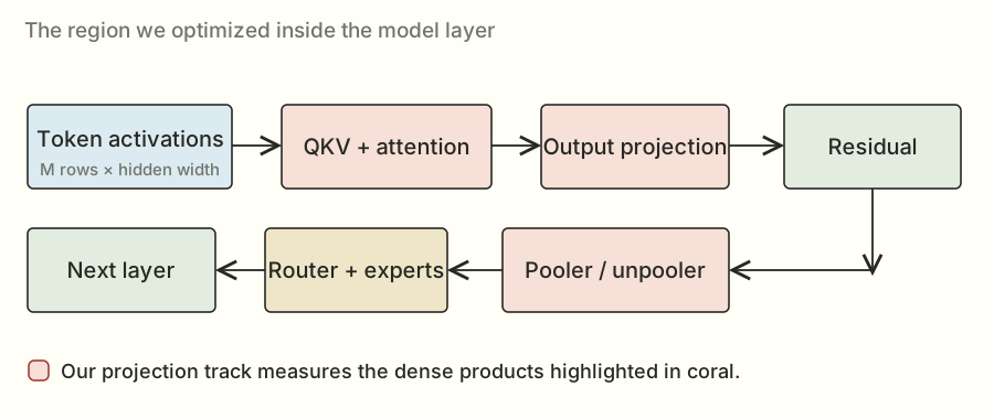
The important thing to keep in mind is that improving one box doesn't make every other box faster. If you speed up the engine of a car, you're still going to wait at a red light. In the model, other calculations, communication, and serving overhead still take time.
There's also a full model walkthrough in my longer notes. I'll connect the main pieces here before narrowing the story to projections.
How those matrices fit into a language model#
I don't want “the model” to remain a mysterious box around the kernels. Here's the path from text to the projection work, without assuming you've studied a transformer before.
A tokenizer maps pieces of text to integer IDs. A token ID is an index into an embedding table: a learned table of vectors. Looking up that row gives the model a numerical starting representation for the token. The ID itself is not a ranking of meanings; token 500 is not inherently twice as meaningful as token 250.
Inside a layer, the input representations are called activations. The model's weights stay fixed during inference, while the activations depend on the current request and the computations before them. This distinction is why I can prepare a weight layout once but must compute a new answer for each new input.
Attention: use other tokens' information#
Attention forms query, key, and value representations, usually abbreviated Q, K, and V. A query represents what a position is looking for; keys provide something to compare it against; values provide the information to combine. These are useful descriptions of the role of the numbers, not literal English questions written into a vector.
For a small numerical illustration, let a query be [1, 0] and two keys be [2, 1] and [0, 3]. Their dot products are 2 and 0. An actual attention implementation applies its specified scaling and masking before converting eligible scores into weights. Here I'll treat 2 and 0 as already-scaled illustrative scores.
Softmax converts scores into positive weights that sum to one. It exponentiates each score and divides by the sum of the exponentials. To make the arithmetic more stable, I can first subtract the largest score from every score. This leaves the normalized result unchanged in exact arithmetic because it multiplies every exponential by the same factor, which cancels in the division.
The exponential is written eᵗ, where e is about 2.71828. At zero it is one; at negative two it is 1/e², about 0.1353. It turns these scores into positive numbers before the normalization. Softmax isn't just dividing the original scores by their sum: original scores can be negative, and their sum can be zero.
For scores [2, 0], subtracting 2 gives [0, -2]. The exponentials are about [1, 0.1353], so the normalized weights are about [0.8808, 0.1192]. If the two value vectors are [10, 0] and [0, 20], their attention-weighted sum is about [8.808, 2.384].
That example shows three different operations: dot products make scores; a nonlinear normalization makes probabilities; a weighted sum combines values. My dense QKV projection helps create the Q, K, and V representations. It isn't the entire attention calculation.
The K in “key” and the K in the GEMM dimension are two uses of the same letter. In the projection equation, K always means the input/reduction width. Context decides which meaning is intended.
Masks and the key/value cache#
When generating text, a token must not use information from future tokens. A causal mask excludes those future positions from its attention. Sliding attention also limits which past positions are eligible. These are part of the required computation, not optional speed tricks.
Previously computed keys and values can be stored in a KV cache and reused on later generation steps. That avoids recomputing the old token representations for every new token. A paged cache adds a table mapping logical sequence positions to physical memory locations, so the kernel must preserve both the numerical values and the addressing rules.
This is also why speculative verification is more than “a bigger batch.” When checking several proposed tokens, each query has its own allowed history and prefix. An implementation can't casually let the first new query read later proposed tokens.
Experts: another use of matrix products#
A mixture-of-experts block uses router scores to choose a subset of expert networks for a token. The selected expert computations still contain matrix products. They also contain nonlinear operations and, in this task, specified normalization and weighting steps.
One common pattern produces a gate vector and an up vector, transforms the gate with a nonlinear function, multiplies the two vectors elementwise, then applies another matrix product. Notice that elementwise multiplication has returned: each gate entry multiplies the corresponding up entry. It does not sum all the features into one dot product at that point.
The nonlinear function means I can't generally push that elementwise work through a matrix multiplication as if everything were one linear map. Fusing operations is useful only if their dependencies and numerical meaning survive.
The routed-expert track used its own weight representation and rules. My dense-projection track preserved its original BF16 dense weights and the allowed router scheme. A technique allowed for a quantized expert problem doesn't automatically become a legal dense-weight approximation.
Normalization and residuals also cost time#
RMS normalization computes a scale from the mean of squared features in a row, with a small specified epsilon for stability, then rescales the row. For [3, 4], the mean square is (9 + 16)/2 = 12.5, and its square root is about 3.5355. Ignoring epsilon and learned scaling just for this illustration, dividing by that gives about [0.8485, 1.1314].
That is different from subtracting the average of the row. The operation's exact position matters too: normalizing individual expert outputs before combining them generally differs from normalizing their combined sum.
A residual connection adds an earlier representation back to a transformed representation. Elementwise addition looks cheap beside a large matrix product, but reading and writing the arrays still takes time. When the matrix products become faster, surrounding operations can become a larger fraction of the remaining total.
Prefill, decode, and running across GPUs#
Prefill processes the prompt and sets up information used by later generation. Decode repeatedly produces the next token. Prefill often supplies many token rows for a matrix product. A lightly batched decode step may supply very few. That's one reason an implementation that likes large matrix products can be awkward for decode.
The full model also uses tensor parallelism across GPUs. For a row-partitioned weight matrix, a GPU can compute a subset of output features. For a split input/reduction dimension, GPUs may instead produce partial contributions that need combining. The exact partition is specified by the model and task.
Our projection shapes are the local shapes supplied under that partition. A thread-block cluster inside one H200 is not the same thing as eight GPUs cooperating across the node. I'll use “cluster” for the on-GPU block cooperation in the kernel story; the full serving system has a larger communication problem around it.
That is enough of the surrounding model to see the stakes. A projection kernel is a repeated numerical building block. It needs to deliver the right numbers to the next operation, and a kernel speedup has to survive integration before it can become a measured serving improvement.
How the Python file turns into GPU work#
The submission was a Python file, but that doesn't mean a Python interpreter performed every multiply in the inner loop. Several pieces of software connected the file to GPU instructions.
PyTorch supplied tensor objects, allocations, library calls, and utilities for building native extensions. A tensor includes its data, shape, strides, device, and dtype. Two tensors can have the same logical shape and values while using different strides or memory locations.
When I write a matrix product in a framework, it can dispatch to an optimized GPU implementation. The framework call is a way to request work; the heavy arithmetic happens on the device. The SGLang baseline already selected useful paths, which is why replacing it with a compact custom kernel wasn't an automatic improvement.
Triton let me express tiled loads, arithmetic, and stores in a Python-like kernel language. Its compiler turned that description into device code. A compiler translates a higher-level program into lower-level instructions. Triton's @triton.jit marks a kernel for just-in-time compilation, and compile-time parameters can specialize the generated code for tile sizes, dtypes, and known dimensions.
That specialization is useful: if a loop bound or tile size is known, the compiler can arrange and simplify the work differently. It also means a large search may compile many variants. Compilation takes wall-clock time even when it is outside the reported steady-state kernel score.
CUDA C++ and inline device instructions gave the native cluster kernels more explicit control over staging, matrix fragments, and block cooperation. The submission embedded native source and built it through the installed extension mechanism. This kept the artifact within the one-file interface while still producing GPU machine code.
cuBLASLt and FlashInfer supplied existing implementations for selected regions. Calling a library wasn't giving up on optimization; choosing a better valid call or retaining a strong library route was part of the final program's design.
The environment mattered because the available APIs, compiler behavior, algorithms, and supported architecture features depend on it. The saved lab record used the prescribed SGLang development image, PyTorch 2.14.1 with CUDA 13, and Triton 3.8. Those are historical environment details for this investigation, not a recommendation to install those versions blindly today.
Preparation and warmup got the needed representations and compiled paths ready before the measured replays. The whole official run still had a finite time budget: the saved task allowed ten minutes including compilation, so an enormous source-generation or compilation search could time out even if one eventual kernel might be fast.
There was also a separation between the lab and the submission. I used SSH, synchronization scripts, and Runpod to run experiments remotely. The evaluated file itself had to operate inside the provided offline environment. Renting the GPU and moving logs around were experiment infrastructure; they weren't actions taken inside the timed kernel.
The same calculation shows up in different sizes#
Here's the compact mathematical version of the weighted sums:
X is the input table. W is the weight table. Y is the output. The little ᵀ means transpose: swap a table's rows and columns so the dimensions line up for multiplication.
There are three sizes I'll keep mentioning. M is how many token rows I'm processing together. K is how many numbers are in each input row. N is how many outputs I need per row. If those letters get annoying, read them as “tokens, input width, output width.”
The competition tested six groups of work, called loads. Three were decode cases: generating with 1, 16, or 32 token rows. The other three were verification cases, where the model checks several proposed tokens together. Those had 8, 128, or 256 rows.
Each load contained five projection families. So there were thirty scored shapes altogether. A shape is just a particular combination of those sizes.
| Projection | N | K | Weights |
|---|---|---|---|
| QKV + gate | 2,304 | 8,192 | BF16 |
| Output | 8,192 | 1,024 | BF16 |
| Pooler | 4,096 | 8,192 | BF16 |
| Unpooler | 1,024 or 8,192 | 4,096 | BF16 |
| Router | 256 | 8,192 | FP32 |
N is the output width; K is the input width. BF16 and FP32 are number formats, explained a little further down. The unpooler uses a smaller output slice for the task’s small-token cases.
The table now has a precise mathematical meaning. For QKV, one token row with K = 8,192 features must produce N = 2,304 outputs. For pooler, the input width is still 8,192 but the output width is 4,096. Those different dimensions create different amounts of work and different useful tile grids.
The weights stay fixed during these runs, so the task let me prepare useful arrangements of them before the timed calls. The actual token inputs still arrived fresh. This is what made later weight-packing experiments possible: I could organize the ingredients ahead of time, then do the input-dependent calculation when asked.
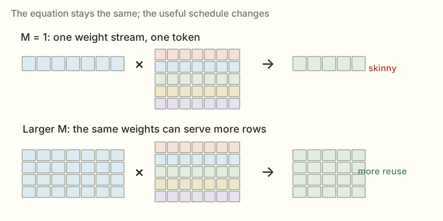
At one token, I read a weight and use it for that one row. With more token rows, I may be able to reuse the same weight for several rows before fetching it again. That reuse can make a different implementation worthwhile.
Imagine getting a book off a shelf. If you're answering one question, you might grab the relevant page and put it away. If you're answering a hundred related questions, keeping the book open makes more sense. The GPU version has more rules, but the reuse idea is similar.
This is why I stopped looking for one kernel that would win everywhere. I needed different approaches for different sizes.
A quick guide to the numbers I'll be showing#
The speedup is baseline time ÷ my time. If the baseline takes 10 microseconds and my version takes 8, the ratio is 1.25×. A microsecond is a millionth of a second. Tiny on its own; useful when a model repeats these operations constantly.
There were also two kinds of official run. A check tested correctness and performance without putting the result on the leaderboard. A scored submission made a leaderboard attempt. They were separate evaluations and sometimes returned slightly different numbers.
Here's the short version of the route. These are selected milestones; I'll get into what changed below.
| Candidate / change | Evidence | Speedup |
|---|---|---|
| 001 · First candidate | check | 0.7761× |
| 002 · Split router | scored | 1.1037× |
| 004 · Shape-aware router dispatch | scored | 1.1144× |
| 009 · Packed high/low router | scored | 1.1555× |
| 026 · Expanded method bundle | scored | 1.1993× |
| 029 · Measured best-of plan | check | 1.2564× |
| 030 · Atomic router | scored | 1.2785× |
| 033 · Cluster QKV | scored | 1.2888× |
| 036 · Streaming vector + selected layouts | scored | 1.3012× |
| 039 · PDL + library choices + skinny QKV | scored | 1.3234× |
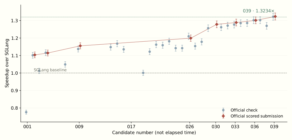
The line makes this look more orderly than it felt as an engineering problem. There were plenty of branches between those points. Some ran correctly and were slow. Some didn't run at all. I kept both kinds in the full experiment log.
One more wrinkle: the final competition number combines the six loads. Inside a load, it adds the five projection times with the specified weights. Then it combines the six speedup ratios using a geometric mean: multiply the ratios and take the sixth root.
Why do that? Consider a simpler example with two loads. Make one twice as fast and the other half as fast. Their ratios are 2 and 0.5. Multiplying gives 1, so the geometric mean is 1: no overall win by that measure. An ordinary average would give 1.25 and make that trade look much nicer than it is.
You can play with one load here while leaving the other five unchanged:
Change one load’s speedup. The other five are held at 1.00×.
Illustrative calculator, not a prediction of a kernel’s performance.
My eventual 1.3012× result worked out to about 23.15% less aggregate time. The later 1.3234× result worked out to about 24.44% less time. The speedup ratio and the percentage of time saved are different ways of describing the same improvement.
Within load ℓ, the ratio is the weighted baseline time divided by the weighted candidate time. All five projection families have listed weight 62 in this task, so that common factor cancels. The overall result is the geometric mean of the six load ratios. The 036 result reports 4,830.8 μs for the baseline aggregate and 3,712.563851 μs as the candidate's score-equivalent time. These combine workloads; they aren't the time of one GPU launch.The exact scoring formula, if you're curious
S = exp((1/6) Σℓ=1…6 log Sℓ)
Having lots of workers doesn't help if I give them nothing to do#
The GPU I used was an H200. The first thing worth understanding about it is that doing arithmetic and getting the numbers to that arithmetic are separate jobs.
You'll also see the name Hopper. That's the architecture family this GPU belongs to. Some of the later techniques use features introduced with that family.
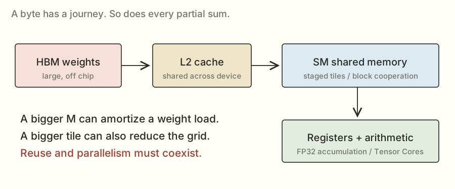
The weights live in a large memory called HBM. Closer to the computation are smaller, faster places to keep data: a cache called L2, shared memory that cooperating threads can use, and registers that hold values used by individual threads.
A thread is one execution path through the kernel. Threads run in groups of 32 called warps. Several warps can belong to a block. Blocks are scheduled onto the GPU's processing units, called streaming multiprocessors, or SMs.
You don't need that whole hierarchy memorized. For the next experiment, the important bit is that separate blocks give the GPU independent pieces of work to schedule. A huge amount of work trapped inside a small number of blocks can leave other parts of the GPU with nothing useful to run.
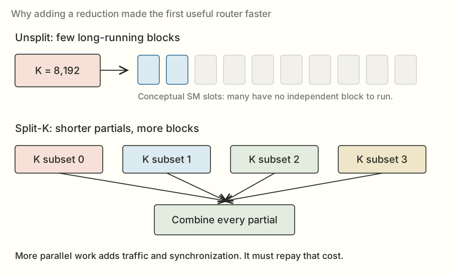
That's roughly the problem identified in the notes for my first router implementation. The router computes scores used to select experts. It had only 256 output features, but each output involved a long sum over K = 8,192 inputs. At small token counts, the chosen output tiles produced too few blocks.
It was a bit like having a large team available and handing out only a couple of enormous tasks. The tasks got done correctly. The rest of the team couldn't do much about how long they took.
That first candidate, 001, passed correctness and checked at 0.7761×. The next idea was to break up the long sums.
Before the first win, I want to make the memory and scheduling part as concrete as the algebra. It explains why a mathematically identical program can take such a different amount of time.
What a matrix looks like in memory#
The GPU doesn't see a pretty rectangular table. It sees memory addresses. The table's shape and strides tell the program how to turn a row and column into an address.
For a contiguous row-major matrix W with shape [N, K], rows sit one after another. The entry W[n, k] is n × K + k elements from the beginning. If each element occupies two bytes, the byte offset is 2 × (n × K + k).
For the small weight matrix from the earlier example, the stored sequence is:
Logical rows:    [ 4, -1 ]  [ 1, 2 ]  [ -2, 3 ]
Flat storage:      4  -1      1  2      -2  3
Element offset:   0   1      2  3       4  5
A stride is the distance, in elements, required to move one step along an axis. This W has row stride 2 and column stride 1. Its transpose can be described as shape [2, 3] with strides [1, 2], using the same underlying storage. A contiguous copied transpose instead stores 4, 1, -2, -1, 2, 3 in a new array. Same logical transposed matrix; different storage order.
That distinction is why “I transposed it” isn't a complete performance explanation. I need to say whether I changed the view, made a copy, or packed values into a tile-specific arrangement, and which addresses the timed kernel will actually read.
Coalescing: think about a group of lanes' addresses#
GPU memory is transferred in chunks. If neighboring lanes request neighboring values, the hardware can service them using a compact set of memory sectors. This is coalescing. A scattered request can require more sectors to deliver the same useful data.
For an aligned illustrative read of 32 FP32 values, one per lane, the useful payload is 128 bytes. Consecutive addresses cover four 32-byte sectors. If those 32 lanes instead touch widely separated locations in distinct sectors, the request could need 32 sectors for the same 128 useful bytes. Cache reuse and the actual instruction path can change the traffic, but the address calculation explains why the access pattern matters.
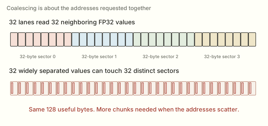
This is a group property. A lane reading values sequentially over time doesn't guarantee that the whole warp's reads are coalesced at one instruction. I have to inspect what all the active lanes request together.
The original W layout makes consecutive K entries in one row adjacent. A different kernel might want adjacent output features at one K step. Those are separated in the original layout. Packing can put the values that the kernel consumes together next to each other without changing their numerical values.
Tiling: load a small piece and use it more than once#
Suppose a block computes a 2 × 2 output tile, and I consider two K terms at a time. It needs a 2 × 2 input tile and a 2 × 2 weight tile: eight distinct operand values. Those values contribute to eight multiplications across four output cells.
If I computed each output cell separately and fetched both operands for both of its K terms without reuse, I'd request sixteen operand values. Cooperative tiling lets neighboring outputs share the values they have in common. This little count illustrates reuse; a real baseline may already benefit from caches and more sophisticated tiling.
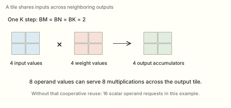
For general tile sizes BM, BN, and BK, a K step brings in about BM×BK + BK×BN operand elements and performs about 2×BM×BN×BK useful floating-point operations. With two-byte BF16 operands and ignoring other traffic, the ratio is BM×BN / (BM + BN) FLOPs per operand byte for that tile step.
Larger output tiles improve that simplified reuse ratio. But they also need more accumulator state and operand storage. If a block owns too much work, fewer blocks may fit on an SM or the grid may have too few independent blocks. Tiling is a balancing problem, not a proof that the biggest tile wins.
Use the real pooler dimensions M=16, N=4,096, K=8,192, and change an illustrative output tile.
Full-tile operand reuse model: 10.67 FLOPs per BF16 operand byte.
Geometry calculator only. These are not measured configurations or a runtime prediction. The model ignores scratch, outputs, cache effects, instruction granularity, and scheduling costs.
There are several levels of tiling. Blocks own output regions. Warps cooperate on smaller regions. Threads hold parts of the accumulators in registers. Reusing a value from a register can avoid repeatedly loading it from shared memory, just as shared-memory reuse can avoid repeatedly fetching it from a farther-away level.
Shared memory has a layout problem too#
Putting data in shared memory doesn't make every access equally cheap. It is organized into banks. In the usual 32-bit-word view of NVIDIA shared memory, a useful simple model has 32 banks with successive words mapping to successive banks. Requests for different addresses in the same bank can need extra servicing. Multiple lanes reading the same address are a broadcast case, which is different from a conflict among distinct addresses.
For a concrete layout calculation, let lane j read word 32×j. Its bank index is (32×j) mod 32 = 0, so all those distinct words land in one bank. Add padding so the stride is 33 words and the bank index becomes (33×j) mod 32 = j for lanes 0 through 31. The logical values can stay the same while the bank mapping changes.
Real matrix-load instructions and wider accesses have additional details. This example explains the purpose of padding and swizzling: alter the address layout so the intended cooperative read pattern works better. It isn't a reason to change an arbitrary array's stride and assume performance improved. I still need the exact consuming instructions and a timing.
Enough active work, with enough resources#
An SM has finite registers, shared memory, and thread capacity. A block that needs more of one resource can reduce the number of blocks resident at once. Occupancy measures active warps relative to the hardware's maximum, but occupancy is only part of the picture.
More active warps can help hide a wait by giving the scheduler other work to issue. A kernel with enough instruction-level work may also make good progress at lower occupancy. Meanwhile, high occupancy doesn't compensate for a scattered memory pattern or too much redundant traffic.
That is why the statement “the GPU was underused” needs a mechanism. Was the grid too small? Were resources limiting residency? Were warps waiting on data? Was arithmetic padded away on invalid token rows? Timings can show a candidate lost; counters and controlled experiments help identify which explanation is right. I didn't have those counters on the Runpod host, so I kept the difference between a measured outcome and a plausible cause.
The CUDA Best Practices Guide is the reference for coalescing and shared-memory access rules. The numerical layouts above are my small worked examples.
A rough way to ask how much room was left#
Before spending another round on a kernel, I wanted a rough sense of what could be limiting it. The roofline idea compares useful arithmetic with data movement.
There are about 2MNK floating-point operations in a matrix multiplication by the usual counting convention: multiply and add count separately. For an individual dot product starting without a zero accumulation, the exact scalar count can be K multiplies and K−1 adds. The conventional 2MNK count is useful for throughput comparisons; it isn't a count of GPU instructions. One matrix instruction can do many of those operations at once.
If a computation needs F FLOPs and the applicable compute throughput is P FLOPs per second, F/P is an optimistic compute time. If it must move B bytes through a memory level with bandwidth Q bytes per second, B/Q is an optimistic movement time. If movement and compute overlap, a simple lower-bound model is their maximum, not automatically their sum. Dependencies and overhead can make the real time larger.
For the pooler with M = 16, N = 4,096, and K = 8,192, the BF16 weight payload is:
2 × 16 × 4,096 × 8,192 = 1,073,741,824 FLOPs
That's 64 MiB of weights, or about 67.1 decimal MB. A MiB is 1,048,576 bytes; a decimal MB is 1,000,000. I keep that distinction explicit when dividing bytes by a bandwidth quoted in decimal units.
Using the simplified assumptions in my saved derivation—4.8 trillion bytes per second and 989 trillion applicable operations per second—the weight-only movement bound is about 13.98 μs, while the arithmetic bound is about 1.09 μs. Those are optimistic model inputs, not a measurement that my kernel reached either peak.
The task's own floor calculation includes input and output traffic as well as weights. This deliberately simpler weight-only calculation isolates why the large fixed weight stream matters, so its number can differ slightly from the full task floor.
Now change only M to 256. The original weight matrix has exactly the same byte size, but useful arithmetic grows sixteenfold. The simplified compute bound becomes about 17.37 μs. The balance changes even though the layer name stays “pooler.”
Divide 2MNK by the weight payload 2NK, and the result is M FLOPs per weight byte. That's the weight-only arithmetic intensity. It ignores activations, outputs, scratch, metadata, rereads, and access inefficiency. It is useful for understanding why token count changes the regime, not for claiming I measured the actual HBM traffic.
The handoff also had empirical read probes: about 3.84 μs for 8.4 MB, 5.79 μs for 16.8 MB, 10.43 μs for 37.7 MB, and 16.65 μs for 67 MB. These were observed timings in that lab, not universal hardware limits. They gave me a practical comparison point alongside the ideal arithmetic.
If a weight-streaming path is already near a useful measured floor, doubling its arithmetic throughput might save very little. If it is far above that comparison point, there may be scheduling, traffic, or overhead worth investigating. Neither observation tells me a particular new kernel will win. It helps me choose a question worth testing.
My first useful win: split up the sum#
Suppose I need to add up a long list of products. Instead of giving one group the whole list, I can give several groups different pieces. Each computes a partial sum. Then I add the partial sums together.
That's split-K. The K dimension is the long input dimension, and I'm splitting the work along it.
A reduction, worked out with small numbers#
A reduction combines a collection of values into fewer values, often by adding them. The dot product's final sum is a reduction. The output can be one scalar even when thousands of input terms contribute.
Use this small dot product:
w = [5, 6, 7, 8]
x · w = 5 + 12 + 21 + 32 = 70
One split could compute the first two terms, getting 17. A second could compute the other two, getting 53. Add their partials and the answer is still 70 in exact arithmetic. The real router used an interleaved K-tile assignment; this contiguous two-piece example is just the simplest way to see the mathematical identity.
The important requirement is that every intended K term is included exactly once. Overlapping splits would double-count work; missing a split would drop terms. Masks also have to exclude padded entries without excluding valid ones.
How splitting changes the grid#
For a tile-based output kernel, a simplified block count is ceil(M/BM) × ceil(N/BN). ceil means round up: seventeen rows with a sixteen-row tile need two tiles, not one. A split axis with S pieces can multiply that grid by S.
Consider an illustrative router with M = 16, N = 256, BM = 16, and BN = 64. The unsplit output grid has 1 × 4 = 4 blocks. Thirty-two splits would expose 128 blocks. That is a large scheduling change even though the mathematical output still has only 16 × 256 = 4,096 numbers.
These are example settings to explain the count, not a claim that every candidate used them. The selected plan in each source names the actual split and tile settings for that range.
More blocks do not create more useful mathematical work. They redistribute the same reduction and add some overhead. The win depends on how much idle capacity this redistribution makes useful, how much work remains per block, and how expensive the final combination is.
The temporary array is a real cost#
With S = 32 splits, M = 16 token rows, N = 256 outputs, and four-byte FP32 partials, the temporary has:
Writing those partials once and reading them once is about one MiB of payload traffic, before other accesses or transaction inefficiency. The combine kernel has its own launch and execution costs. Cache behavior can affect where traffic is served, so payload counting is not a bus-counter measurement.
At a large M, there may already be many output tiles. Splitting can still add scratch and synchronization without solving a shortage of blocks. That explains why “split more” was a hypothesis for a regime, not the direction of unlimited improvement.
Why a last-block scheme was more complicated than it sounded#
One later idea let blocks write partials and update a completion counter. The last block to arrive would read the others' partials and finish the output, avoiding a separate final launch.
But a counter is not enough by itself. The final reader needs the partial writes to be visible before it reads them. The protocol has to use the right ordering and synchronization, and every replay needs a fresh counter. Otherwise the code can work once and fail later or read unfinished data.
Even a correct protocol still writes partials, updates counters, waits for readiness, and reads the partials back. Avoiding a launch is useful only if those costs are better than the path it replaces. The tested last-block variants did not beat the atomic incumbent.
No. The per-split arithmetic may shrink, but launch, scheduling, scratch traffic, and combination costs don't shrink the same way. Too many tiny pieces can leave more coordination than useful work. The best split count depends on the shape and the full implementation.Pause: if I double the split count, does the runtime halve?
In candidate 002, small-token router ranges used sixteen splits. Each block worked on its assigned K tiles and wrote its partial answer into a temporary GPU array. A second kernel added the partials to produce the final output.
Notice the trade: I added a temporary array, extra memory traffic, and another launch. Launching a kernel means asking the GPU to start that program, which has a cost of its own. The hope was that having more useful blocks running would save more time than the extra steps cost.
It did. The official check returned 1.1014×, and the scored submission returned 1.1037×.
That was the first useful lesson: a program with more steps can finish sooner if those steps let the hardware work more effectively.
Show me the actual split-router code
def _router(X, HI, LO, Y, M: tl.constexpr, N: tl.constexpr, K: tl.constexpr,
            BM: tl.constexpr, BN: tl.constexpr, BK: tl.constexpr, SPLIT: tl.constexpr):
    rows = tl.program_id(0) * BM + tl.arange(0, BM)
    cols = tl.program_id(1) * BN + tl.arange(0, BN)
    kk = tl.arange(0, BK)
    hi_acc = tl.full((BM, BN), 0, tl.float32)
    lo_acc = tl.full((BM, BN), 0, tl.float32)
    for start in range(tl.cdiv(K, BK * SPLIT)):
        k = (start * SPLIT + tl.program_id(2)) * BK + kk
        x = tl.load(X + rows[:, None] * K + k[None, :],
                    (rows[:, None] < M) & (k[None, :] < K), other=0)
        offsets = k[:, None] * N + cols[None, :]
        mask = (k[:, None] < K) & (cols[None, :] < N)
        hi = tl.load(HI + offsets, mask, other=0)
        lo = tl.load(LO + offsets, mask, other=0)
        hi_acc += tl.dot(x, hi)
        lo_acc += tl.dot(x, lo)
    tl.store(Y + tl.program_id(2) * M * N + rows[:, None] * N + cols[None, :], hi_acc + lo_acc,
             (rows[:, None] < M) & (cols[None, :] < N))
But the win wasn't uniform. The smaller-token router cases benefited, while the 256-token case regressed. At larger token counts, there was already more independent output work. Splitting K still charged me for combining partial answers, even when I needed its parallelism less.
So the next question became: where should I use this, and where should I leave the existing path alone?
Reading the split-router kernel with the equation beside it#
The short source excerpt can look dense if Triton is new, so I'll connect it back to Y[m,n] = Σₖ X[m,k]W[n,k].
tl.program_id(0) identifies which token tile this program owns. Multiplying it by BM and adding tl.arange(0, BM) makes a vector of token-row indices. The second program ID does the same job for BN output columns. The third program ID identifies the K split.
tl.arange describes a logical array of indices for the compiler. It does not launch that many independent CPU threads. Triton maps these logical elements and their operations onto the GPU program's warps and lanes.
Now look at the K-index expression: (start * SPLIT + program_id(2)) * BK + kk. For the 002 small-token router settings, BK is 64 and SPLIT is 16. Split zero handles K positions 0–63 on its first loop step, then 1,024–1,087 on its next. Split one begins with 64–127, then 1,088–1,151. Across all sixteen splits and eight loop iterations, the 8,192 K positions are covered.
Each loop loads an input tile of shape [BM, BK] and two weight tiles of shape [BK, BN], one for the high contribution and one for the low. Two dot products update FP32 accumulators of shape [BM, BN]. After the local K work, the program stores its combined partial in the slice owned by its split.
The mask arguments say which logical entries are valid. A token tile of sixteen rows may be used for a smaller actual M. Those extra rows must not load or store outside the intended array. Masked values can be supplied as zero for the arithmetic, but the implementation must still write all valid outputs.
The following sum kernel walks the split axis, adding every partial for each valid output cell. Its mathematical role is exactly the little 17 + 53 = 70 example. Most of the complexity is now about assigning addresses and work, rather than changing the operation.
Why an empty scratch buffer could be okay here#
The split path allocated its partial tensor without filling it with zeros. That's valid only because each required partial location is freshly written by its owner before the sum kernel reads it. The previous contents don't contribute.
The atomic path is different: a block reads-modifies-writes a shared destination by adding to what is already there. Its starting contents are part of the answer, so they must be initialized correctly. “This allocation can be empty” is a property of how the kernel uses it, not a general performance rule.
Preparation is not secretly computing the answer#
The task separated prepare(weights) from the timed entry point. Preparation could transpose or pack fixed weights, compile extensions, and reserve reusable state. It did not receive the evaluated activations needed to compute their outputs.
For example, packing W into output-feature tiles preserves information I will need for any future X. Precomputing Y for an input I haven't received is impossible without changing the problem. Reusing Y from a previous X would be wrong. That is the clean boundary behind the layout experiments.
The saved contract gave preparation a finite budget, including up to 300 seconds for that phase. Native compilation also had to fit the overall evaluation lifecycle. A fast method that needed an unbounded search or manual setup outside the allowed environment would not be a usable submission.
Inside the timed call, dispatch could use known shape and configuration. Pulling activation values back to the CPU to decide what to do would introduce host synchronization and conflict with the captured execution requirements. The selected routes used the geometry of the job, not a lookup of evaluated answers.
I started picking a method based on the job#
The word for this is dispatch. It just means “look at the input, then choose which implementation to run.”
At one token, a direct matrix-vector calculation can make sense. That's matrix multiplication with only one input row; you'll see it called GEMV in the code. With more rows, a tiled matrix-multiplication kernel can reuse data. At other sizes, the existing library can be the best choice.
Candidate 003 tried a more selective vector arrangement and checked at 1.0121×. Candidate 004 adjusted the router ranges and selected vector paths more carefully. It scored 1.1144×.
These were whole candidate programs, so I can't subtract one score from another and claim that every bit of the difference came from a single change. What the results did show was that choosing useful regions for different methods was worth pursuing.
This also explains why I'll keep saying “at this size.” A method can be a good answer for sixteen tokens and a poor answer for two hundred and fifty-six. Calling it a good or bad kernel without the size leaves out half the story.
A small detour: the numbers themselves have formats#
Before the next router change, there's one more idea we need: how the GPU stores a number.
FP32 is a 32-bit floating-point format. BF16, or bfloat16, uses 16 bits. Fewer bits mean less storage and different precision. BF16 also works with fast matrix hardware on the GPU, called Tensor Cores.
That doesn't mean I can quietly change every FP32 number to BF16 and declare the program faster. The task still has a numerical contract: rules for how close my answers must be to the reference calculation. The router is especially sensitive because its scores help choose experts.
What a floating-point number is approximating#
The computer has a finite bit pattern for each stored value. A bit is a binary digit, zero or one; eight bits make a byte. An FP32 value occupies four bytes, while a BF16 value occupies two.
A useful way to understand a normal finite floating-point value is binary scientific notation. In decimal, I might write 1.23 × 10³. In binary, the stored parts describe a sign, a power of two, and significant binary digits. The exponent largely determines the scale; the significand determines the detail within that scale.
FP32 has one sign bit, eight exponent bits, and 23 explicitly stored fraction bits. BF16 has one sign bit, eight exponent bits, and seven stored fraction bits. For normal values there's also an implicit leading one. The same exponent width gives BF16 a broad range, but the shorter fraction means much wider spacing between nearby representable values.
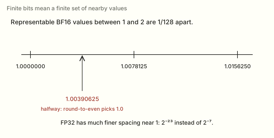
For example, in the interval from 1 up to 2, neighboring BF16 values are separated by 2⁻⁷ = 1/128 = 0.0078125. Some consecutive choices are 1.0000000, 1.0078125, and 1.0156250. FP32 spacing in that interval is 2⁻²³, about 0.0000001192.
The spacing changes with the exponent. BF16 is not “keep a fixed number of digits after the decimal point.” A fixed absolute difference can be tiny at one scale and unrepresentable at another. Zero, subnormal values, infinities, and NaNs have additional representation rules; the task's difficult-input checks matter partly because ordinary values don't exercise every edge case.
Inputs, products, accumulators, and outputs are separate choices#
An accumulator holds the running total while the kernel combines products. A kernel can read BF16 operands, accumulate in FP32, then round the final output into BF16. Those are three different format decisions.
Reading a BF16 value into FP32 doesn't recover information that was already lost when the original value was rounded into BF16. It does let later arithmetic use the wider format. Likewise, a BF16 output tensor doesn't prove intermediate partial sums were combined in FP32; a library might have multiple allowed reduction schemes.
That is why I checked the library's compute and split-reduction settings as well as the final tensor dtype. For the selected cuBLASLt search I requested FP32 compute and the intended compute-type reduction behavior. The correctness tests still had the final say.
Algebraic rearrangements can change rounding#
In exact arithmetic, addition is associative: (a+b)+c = a+(b+c). Floating-point addition rounds to a finite set of values after an operation, so that equality need not survive.
Take these three values in FP32: 100,000,000, 1, and −100,000,000. The representable spacing around 100 million is larger than one. Adding one to the large positive number can round back to that large number. Subtracting the large number then leaves zero. Cancel the two large numbers first, then add one, and the answer is one.
Both expressions are exactly one in real arithmetic. The computer's finite arithmetic can produce different results because it rounds at different stages. Splitting a reduction or changing which partial arrives first changes those stages. Fused multiply-add and matrix-instruction details can also affect where rounding occurs, so source-level algebra alone doesn't determine the exact bits.
This is not permission to accept any error. The task defines acceptable error against its reference, including row-level conditions and invalid-value checks. An optimization needs to pass that contract across the required inputs.
Why the high-plus-low router scheme helped#
Now I can say more precisely what the high and low parts were doing:
R = W − FP32(H)
L = roundBF16(R)
XWᵀ ≈ XHᵀ + XLᵀ
H captures a coarse version of the original weight. R is the residual left after that approximation. L captures much of that residual on its smaller scale. Since the residual is smaller, BF16 can represent details there that it couldn't preserve beside the original large value.
For a convenient exact binary example, take W = 1.00390625, halfway between two BF16 values near one. With round-to-nearest, ties-to-even, H is 1.0. The residual is 0.00390625, which itself is representable in BF16. Here H + L reconstructs this chosen value exactly.
That example explains the idea, not a universal theorem about every FP32 weight. The residual also gets rounded, and the later products and sums introduce their own numerical behavior. The task explicitly permitted this scheme, and I tested it rather than claiming arbitrary lower precision was equivalent.
Contrast that with lossless packing: if I take a stored BF16 value and move its unchanged bits to another address, there's no new approximation at that preparation step. The new execution order can still affect rounding later, but the representation change itself preserved the weight values.
What a useful correctness check has to catch#
Suppose the input row is zero everywhere except feature j, where it equals a power of two. Each output becomes a scaled entry from weight column j. That is a very direct probe of the weight representation. A bad approximation can't rely on cancellation across thousands of random products to look acceptable.
I also need rows where the true output is small. Relative error divides by a scale, so values near zero require the task's specified handling. Replacing the reference's rule with a convenient average error would change what passing means.
And I need repeated calls with new inputs. Passing the first call says nothing about whether a scratch buffer, output, or counter was reset for the second. I'll return to that lifecycle issue in the atomic router and benchmark sections.
The actual error rule, including what L2 means#
The L2 norm of a vector is the square root of the sum of its squared entries. For [3, 4], that is sqrt(9 + 16) = 5. It's a way to measure the size of the whole vector without letting positive and negative entries cancel. For this whole-output comparison, the array's entries are treated together in the norm.
Relative L2 error divides the norm of the error by the norm of the reference:
If the reference is [3, 4] and my output is [3.03, 4.04], the error vector is [0.03, 0.04], whose norm is 0.05. Divide by the reference norm 5 and the relative error is 0.01, or 1%. That is a whole-vector measure; it doesn't say every individual entry was exactly one percent off.
The saved dense-projection task allowed whole-output relative L2 error up to 1% for the BF16 projections, and 0.01% for the router. The reference performed the matrix product in FP64 and converted to the required output type before the supplied comparison. I used the reference implementation rather than substituting a different interpretation of that rule.
Every row also had to satisfy a bound five times its corresponding tolerance. Its denominator was its own reference norm or, if larger, one tenth of the average row norm, with a small numerical floor. That stops a legitimately near-zero row from making a ratio explode while still constraining each row. Otherwise one bad row could hide inside an acceptable whole-array average.
Sparse probe rows had a separate 0.1% bound. The generator selected them at roughly one row in eight, with at least one at M≥8. The checks also required the exact output shape and dtype and rejected NaN or infinity. Those are different failure modes: the correct shape doesn't excuse the wrong numbers, and a small average error doesn't excuse a broken row or a nonfinite value.
The saved projection reference and comparison code contain the exact rules. All these thresholds are the contract recorded for this investigation.
Pause: does an FP32 accumulator make rounded BF16 inputs exact again?
No. It gives the running total more precision, but it can't recover information that was already removed from the input representation. That's why operand formats, accumulation, and output rounding need to be discussed separately.
The task allowed a particular high-and-low BF16 scheme for the router weights. First I made a BF16 version of the FP32 weight, called the high part. Then I took the leftover difference and made a BF16 version of that, called the low part. I multiplied by both parts and combined their contributions in FP32.
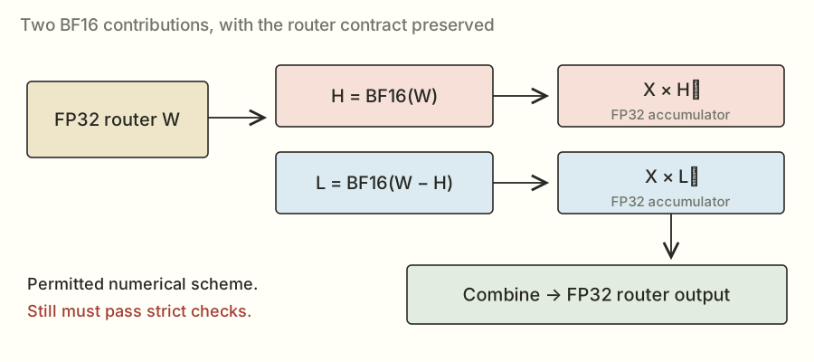
Think of writing down a main amount and a smaller correction. Keeping the correction can improve the result compared with keeping only the main amount. It still has to pass the real tests; two BF16 numbers don't magically represent every possible FP32 value exactly.
The other weight changes I'll describe as lossless packing are different. Those move existing BF16 values to new addresses without changing their bit patterns. Same numbers, different arrangement.
Packing the router got me to about 1.15×#
Candidate 009 arranged the high and low router weights next to each other in a bigger prepared matrix. That let a library multiplication produce both sets of contributions in one call. A small finishing step added the corresponding high and low outputs.
For smaller token counts I kept the split-router path. For a larger range I used the packed library route. I was building a little collection of methods rather than replacing everything with one kernel.
This candidate checked at 1.1372× and scored 1.1555×. The difference between those two numbers was a reminder that check and scored runs are separate measurements. I didn't make another code improvement in between and get to claim the difference as a new technique.
There was still a lot left to do. The bigger dense matrices were reading millions of weights, and their timings made up a substantial part of each load. Making the router faster wasn't going to remove that work.
I also wandered into attention and experts#
This project had a few side quests. They're useful to mention because they explain both what I tried and why the scores can't all be rolled into one big number.
On the attention problem, candidate 005 combined preparation work and scored 1.1323×. A later split variant checked at about 1.1349×.
The routed-expert branch started around 0.9945×, then a version that fused post-normalization work scored 1.1454×. “Fused” means combining work that would otherwise happen in separate steps. Later tile changes reached 1.2684× on that problem. A tile is a small rectangular piece of a matrix assigned to a group of threads.
When validated components were combined into a whole decode layer, candidate 011 scored about 1.0953×. The whole-layer number was smaller than some component wins because other work still remained.
There's a useful formula for this, called Amdahl's law. If half the original time belongs to a part I make twice as fast, the new total time is one half unchanged plus one quarter for the accelerated part. That's three quarters of the old time, or a 1.33× total speedup. It isn't 2×.
I kept these attention, expert, and layer results in their own tracks. The rest of this article returns to projections. The full side stories are in notes 31–33.
Then came a lot of rearranging, measuring, and trying again#
One useful direction was transposing the dense weights ahead of time. The math is equivalent, but the library sees different layouts and may choose a different way to run the product. Candidate 015 checked at about 1.1680×.
Other attempts included a Hopper-specific vector route (014, about 1.1481× checked) and wider K tiles (016, about 1.1353×). A bigger tile can reuse more data, but it can also need more memory or leave fewer blocks to run. “Bigger” wasn't a direction I could just keep turning a dial.
The QuACK library attempts brought a more basic problem. Candidates 017 and 018 failed before giving me useful timings. The interface I was using expected a batch dimension: an extra outer dimension around the input matrices. Adding it in 019 and 020 got the calls working. They then checked at about 1.0009× and 1.1221×.
The source describes those operands as rank-three arrays. In that API, rank means the number of array axes: batch, rows, and columns. It is different from the linear-algebra meaning of matrix rank, which concerns independent rows or columns.
That distinction matters. A program that didn't run hadn't told me the library was slow. It had told me the integration needed fixing.
I then searched groups of settings more systematically: how many output rows a block owned, how many warps it used, tile sizes, split counts, and library plans. cuBLASLt, which shows up a lot in the files, is NVIDIA's matrix-multiplication library interface with more control over layouts and algorithm choices.
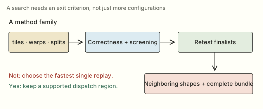
Trying lots of settings creates its own trap. If I pick the fastest single timing from a huge search, I might be picking a lucky measurement. So useful finalists needed more runs, new inputs, and nearby sizes. A setting that works at M = 32 also needs sensible behavior around that boundary.
The combined candidate 026 checked at 1.2099× and scored 1.1993×. Later, the best-of plan in 029 checked at 1.2564×. The Claude handoff helped preserve the useful methods, known failures, and remaining opportunities so the next round didn't have to rediscover all of them.
I was making progress. I was also learning that a bundle of good ideas still needs to be tested as a bundle.
Could I avoid reading all those router partials back?#
Remember split-K? I had lots of blocks producing partial sums, then a final kernel reading and adding those sums. Candidate 030 tried a different way to finish: atomic addition into the final output.
An atomic add is an update the GPU coordinates so two blocks adding to the same location don't simply overwrite one another. Each split can contribute its answer directly.
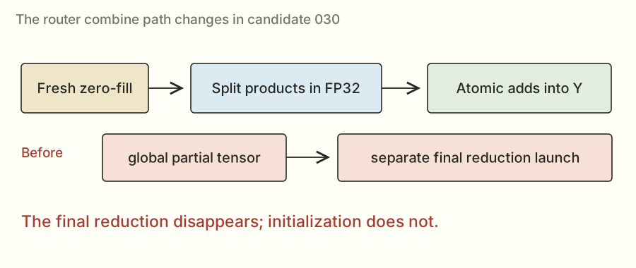
This removed the dedicated final reduction pass, but it didn't remove every extra step. The output still had to start at zero. If I left yesterday's answer in the buffer and added today's answer to it, the result would be wrong. The zero-fill was part of the call I timed.
The code makes that zero-fill explicit
def m_ratomic(x, state, layer, n, k, p):
    bm, bn, bk, split = p[:4]
    tuning = {"num_warps": p[4], "num_stages": p[5]} if len(p) > 4 else {"num_warps": 4}
    m = x.shape[0]
    out = torch.zeros((m, n), device=x.device, dtype=torch.float32)
    _paired_router_atomic[(triton.cdiv(m, bm), triton.cdiv(n, bn), split)](
        x, state["router_interleaved"], out, m, n, k, bm, bn, bk, split, **tuning)
    return out
Floating-point sums can also change slightly when contributions arrive in a different order. Atomic addition doesn't solve that numerical issue for me. I still needed the router's correctness checks.
Follow one output through an atomic router call#
Imagine two splits contribute 17 and 53 to an output. If the output starts at zero, atomic additions make it 0 → 17 → 70, or 0 → 53 → 70 if the other split arrives first. For these small exact integers both orders agree.
If the output instead starts with an old value of 70, the next identical call ends at 140. Each atomic update can be individually coordinated and the complete result can still be wrong. That is why I keep talking about initialization; the atomic operation doesn't decide which computation's answer is currently in the buffer.
A different bug would let two splits each read zero and write their own total without an atomic operation. The final value could be 17 or 53 instead of 70. That's a race: the result depends on conflicting accesses without the required coordination.
Now connect that example back to the real paired router. Each block computes FP32 accumulators for high and low output columns, combines the pair belonging to one logical router output, and contributes its split's result. Masks keep it within valid token and output indices. The final output stays FP32.
Atomic updates can arrive in different orders, so the floating-point rounding example from earlier still matters. The implementation needs acceptable numerical behavior across the task's checks, not an assumption that atomic means bitwise deterministic.
What the code is doing, line by line#
In m_ratomic, the tuple begins with BM, BN, BK, and the split count. Those control the token tile, output tile, K tile, and number of partial contributors. The wrapper gets the current M from the input shape.
torch.zeros((m, n), ..., dtype=torch.float32) creates the initialized output. The launch grid is the number of token tiles, the number of output tiles, and the split count. The kernel receives the prepared interleaved router weights and the fresh input.
The interleaved layout places each output's high and low contributions together. Inside the matrix kernel, the accumulator can be viewed as [BM, BN, 2]; summing that last axis combines each pair. The split still owns only part of K, so it atomically adds the resulting [BM, BN] tile into the final answer.
The complete captured path includes the initialization and the matrix kernel. A profiler row for only the matrix part would not establish the time of the whole correct call.
Why I couldn't just use the same trick for every output type#
The router's required output is FP32. The dense projections return BF16. Replacing an FP32 partial combine with repeated rounding into a BF16 destination changes the numerical path, and suitable fast atomic mechanisms depend on the data type and hardware.
A technique that wins on this router therefore doesn't automatically transfer to every dense matrix. I need both a valid arithmetic path and a favorable complete cost for the target family. The general idea is to examine combination cost; the specific atomic route earned particular router regions.
Candidate 030 scored 1.2785×. That became a stronger starting point for the next experiments.
A tiny matrix and a group of cooperating blocks#
There were two more useful pieces before the 1.30× push.
First, the small-token unpooler uses a smaller output slice. In that region, FlashInfer's tiny GEMM implementation was worth keeping. GEMM is the usual library name for general matrix multiplication. The full candidate 031 checked at 1.2620×, so it wasn't a new overall milestone above 030; its useful piece was a selected method for a particular size.
Second, the small-token QKV projection still had a lot of weight data to read: roughly 37.7 MB. QKV refers to the query, key, and value representations used around attention. For this section, you can think of it as another projection with an awkwardly small token dimension and a long input dimension.
The custom CUDA path split the K work among cooperating blocks and combined their partial results through distributed shared memory. Ordinary shared memory lets threads in a block cooperate. Hopper's thread-block clusters let a selected group of blocks cooperate across their shared-memory regions too.
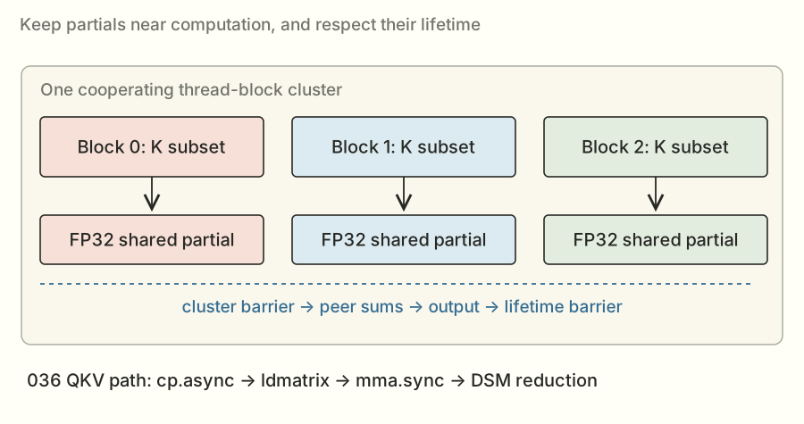
The blocks couldn't just read each other's partials whenever they felt like it. They needed a barrier, a point where they waited until the required work was ready. They also needed to keep that shared storage alive until every reader was done.
This path used cp.async to stage transfers, ldmatrix to load matrix pieces, and mma.sync to do matrix arithmetic. Those names are the deeper implementation details. The larger idea is: move tiles in, compute partial answers, then combine them nearby without a separate global reduction launch.
How a pipeline hides waiting#
Imagine one tile load takes L units of time and computing on that tile takes C. A simple sequential loop spends roughly tiles × (L + C). An ideal overlapped pipeline can approach a startup cost plus one stage every max(L, C) units. That model explains the potential; it ignores contention and synchronization that a real implementation must pay.
For an illustrative four tiles with L = 3 and C = 5, sequential execution would take 32 units. With ideal overlap, loading the next tile during the current computation could finish in about 3 + 4×5 = 23 units. These are made-up teaching units, not timings from my H200.
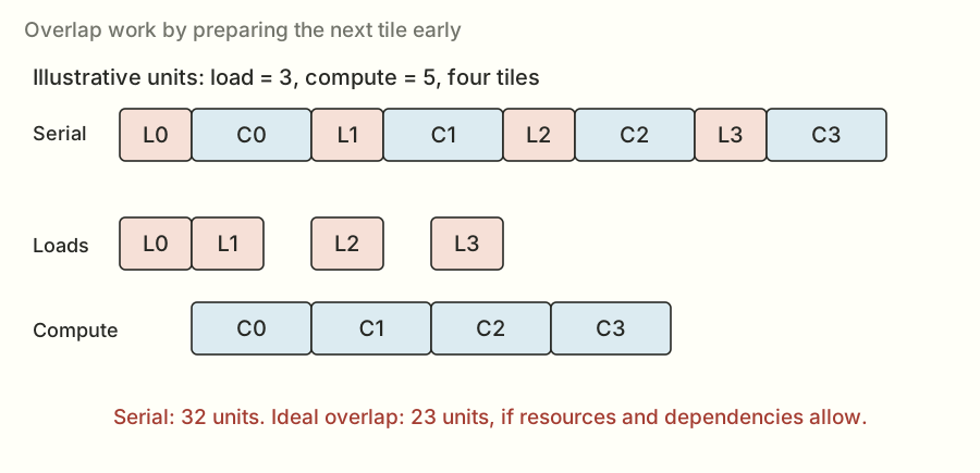
Overlapping requires separate storage for tiles in flight. With double buffering, I can fill one buffer while consuming another, then swap their roles. A deeper stage ring permits more tiles in flight but consumes more shared memory. If a K split has only a few tiles to compute, a very deep pipeline may have little steady-state work over which to repay its startup and resource costs.
That is why adding stages was an experiment. Shared-memory use can reduce residency, and there may not be enough per-block work to make the overlap useful. The deeper QKV sweeps did not establish a useful win over their selected incumbent in that round.
A transfer being issued does not mean the data is ready#
An asynchronous copy lets the program issue a transfer and do other work before waiting for it. The consumer must still wait for the transfer's required completion before using the data. A producer must also avoid overwriting a stage until the consumer is finished with it.
Those are two distinct directions of coordination: ready to read and safe to reuse. A ring of buffers without the right barriers is a race with extra storage around it.
In the earlier QKV kernel, cp.async organized global-to-shared movement. ldmatrix loaded staged fragments into the register organization expected by mma.sync, which updated FP32 accumulators. Several threads or lanes collectively own fragments; the instruction's layout determines which values belong where.
Tensor Core throughput is attractive because one matrix instruction represents many multiply-accumulate operations. It also imposes requirements: supported fragment sizes, compatible formats, properly arranged operands, and correct completion before the accumulators are consumed. Simply translating the scalar loop into a matrix instruction name doesn't supply the surrounding schedule.
Reducing inside a block cluster#
The earlier cluster design distributed K work across cooperating blocks. Each block produced a local FP32 partial, put it into its shared-memory region, and joined a cluster barrier. Peer partials could then be read and summed to form the output.
A later barrier protected shared-memory lifetime. If one block exited or reused storage before another finished reading it, a logically correct reduction formula would still become an invalid execution.
This trades global scratch traffic and a separate reduction launch for cluster cooperation, peer accesses, barriers, and cluster residency constraints. The trade helped the selected skinny QKV regime. It did not remove the need to check whether the whole cluster schedule was actually faster.
Why the later TMA/WGMMA kernel was a new experiment#
TMA can move tensor tiles through a dedicated transfer mechanism, and WGMMA performs matrix arithmetic across a warp group. A producer/consumer organization separates roles: one part of the program keeps future operands moving; another performs the arithmetic on ready operands.
The later 039 skinny path combined those roles with tensor-map loads, shared staging barriers, FP32 accumulation, and cluster reduction. Its selected instances used three K splits and eight stages. That complete arrangement differed from both the earlier cp.async / mma.sync implementation and the earlier losing descriptor-based TMA branch.
I can be more specific from the preserved source. A warp group has four warps, or 128 threads. With the selected MW=1 configuration, the native block has 256 threads: a producer-side group and a consumer group. Thread zero issues the TMA transfers. The consumer group waits for a stage to be full, issues the matrix work, waits for its required completion, and has its warp leaders signal that the stage can be reused. Reserving these roles consumes resources too; the new design still had to earn its timing.
The selected BK is 64, so K=8,192 contains 128 K tiles. The three blocks partition those tiles using integer boundaries: 42 tiles, 43 tiles, and 43 tiles. They need not all do an identical number of tiles, but together they must cover every tile exactly once. This is a concrete difference from a design whose applicability guard requires K to divide evenly by its chosen split width.
The code keeps separate “full” and “empty” stage barriers. Full tells the consumer that the required transfers have completed; empty tells the producer that the previous consumer is done with the slot. Their phase changes let the same ring positions be used across multiple iterations without confusing an old completion with a new tile.
The useful question was not whether TMA “is faster” in isolation. It was whether this layout, role division, pipeline, arithmetic, and combine path beat the prior complete method for those shapes. The official result establishes the later bundle's aggregate outcome; isolating each addition's exact percentage requires the corresponding controlled comparisons.
Candidate 033 independently scored 1.2888×. It kept the cluster method in its useful small-token QKV region and kept other methods elsewhere.
I was close to 1.30×. Getting the rest still took several more branches.
How I checked whether an idea was actually faster#
I edited on my Mac and used a remote Runpod H200 for the GPU experiments. Runpod let me rent the machine; the lab copied source there, ran the jobs, and copied results back. The submitted kernel didn't need internet access.
The timing setup mattered as much as the GPU. If I ran the exact same inputs and weights repeatedly, some data could stay in fast cache. That might tell me more about a convenient replay than the competition's intended workload.
So the lab used new inputs, rotated separate copies of the weights, and cleared out L2 before timing. It also alternated the order: sometimes baseline first, sometimes my version first.
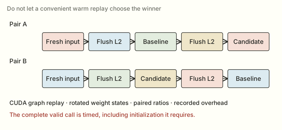
The calls ran as CUDA graphs. A graph records a sequence of GPU operations so it can be replayed with less CPU involvement. Since the judge measured that mode, it was the mode I needed to compare. Timing an ordinary Python call could include different overhead.
The judge also corrected for a fixed replay cost. Locally that correction was recorded at around 4 μs. With operations this short, a small difference in overhead or measurement conditions can move a percentage noticeably.
Correctness wasn't just “try a random input once.” The checks included difficult inputs, unusual values, nearby shapes, and graph replays with fresh inputs. A particularly useful test put one nonzero value in an input row. That exposes a scaled piece of the weights, making it harder for an incorrect weight conversion to hide inside a big random sum.
One limitation: the Runpod host didn't expose the permissions needed for Nsight Compute's hardware counters. I could measure which version won and use timing profiles, but I couldn't claim to have a full counter-based explanation for every loss.
The lab also had an unglamorous cloud-computing lesson: an idle rented GPU can still bill you. The saved notes include an idle billing episode, a credit-related restart failure, and incomplete searches recovered later. Keeping the results locally and checking what actually finished mattered.
What I mean by a fair paired measurement#
A GPU launch is asynchronous: the CPU can finish asking for work before the GPU has finished doing it. A CPU stopwatch around the launch alone can therefore measure the request rather than the computation. The timing path needs the appropriate GPU event and completion handling; the judge's graph-replay benchmark supplied that controlled path.
Suppose the baseline takes 10 μs and my candidate takes 8 μs in one pair. That pair's ratio is 1.25. Another pair might return slightly different times because clocks, scheduling, or the surrounding state changed. Pairing is an attempt to compare nearby observations under similar conditions, and swapping the order reduces a simple first-versus-second bias.
Summarizing several paired ratios is not always numerically identical to taking two unrelated medians and dividing them. I kept the judge's method as the authority for its score and used the local harness to choose candidates worth checking there.
Clearing L2 and rotating weight states also serve specific purposes. Repeating one already-cached weight copy can answer a different question from reading weights under the benchmark's intended conditions. Neither a cold nor warm experiment is universally the right production model; the point here was to match what this competition tested.
A tiny overhead error can look like a useful win#
For a simple illustration, imagine raw event times of 14 μs and 12 μs. Subtract a fixed 4 μs overhead and the adjusted times are 10 and 8, producing 1.25×. Subtract 4.5 μs instead and the ratio is 9.5/7.5, about 1.2667×.
The underlying raw observations didn't change. The adjustment did. This isn't an explanation proven for the local-to-official gap; it's a numerical example showing why very short calls need careful calibration and why a local result near the target wasn't a guarantee.
Longer measurements can reduce some timer sensitivity, but changing the execution mode or removing required work would create a different benchmark. I needed the correct captured call, enough repetitions, and the same comparison method.
Fresh graph replay is a correctness test too#
A CUDA graph records work to replay. It doesn't entitle the implementation to keep an old evaluated answer. If I change X between replays, Y must follow the new X.
The tiny matrix example makes this easy to see. The first input row [2, 3] produces [5, 8, 5]. A later input row [3, 1] must produce [11, 5, -3]. A graph that keeps returning [5, 8, 5] is stale, even if it has an impressively short timing.
The same reasoning catches partial buffers and counters that weren't reset. Eager execution can hide a lifecycle mistake if I only check one call. Replaying with new inputs exercises whether the captured structure still performs the right computation each time.
Search noise changes how I pick a winner#
If I test a thousand configurations, one can look unusually fast by chance. Choosing it from its single best run overstates what I learned. That's why the search was a funnel: cheap screening first, more repetitions for promising candidates, fresh correctness, neighboring shapes, then the complete combination.
Overlapping reported intervals don't prove two programs are identical, and a higher point estimate doesn't prove a tiny difference is repeatable. The right response depends on the size and consistency of the evidence. For a clean dispatch, a clearly useful region is easier to justify than continual changes based on very small noisy differences.
When the official record gives an interval, I show it with the point estimate. When an unfinished search gives only a source file or partial log, I keep it unfinished. Those distinctions are part of the technical explanation, not paperwork after it.
Sometimes moving the same numbers around was enough#
The pooler was another projection where small-token timings left room to improve. Pooler and unpooler are the task's names for two of the surrounding transformations; for the optimization here, their input and output sizes are what matter. The C2 experiments packed the weight values so each output tile's region was contiguous: the values it needed were next to each other in memory.
Imagine having all the ingredients for one recipe together instead of walking up and down the same aisle to find each one. The actual GPU access rules are more precise, but that's the motivation behind this layout change.
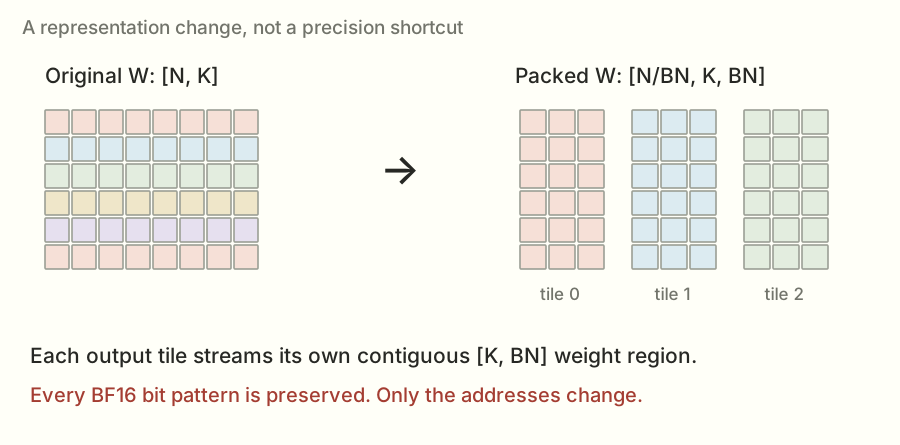
The selected small-token settings used output tiles of 32 features and K tiles of 512, with different token tiles and pipeline depths. A pipeline tries to fetch a future tile while computing the current one. More stages can help overlap, but each stage needs storage, so deeper isn't automatically better.
Local retests showed useful pooler gains. The combined candidate 034, though, checked at 1.2852×, below the earlier scored point for 033. A faster component hadn't yet given me a better official overall result.
I also tried presenting equivalent products to cuBLASLt in different orientations. One way computes the normal product. Another uses prepared transposed weights. Another computes a swapped product and views the output with rows and columns exchanged.
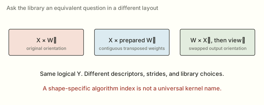
Same logical answer, different library choices. Some were useful at a tested size and poor at a neighboring one. For selected swapped-output routes, token counts not divisible by eight fell back to the retained method because the memory alignment wasn't suitable. Alignment means where data starts and how rows line up with the boundaries the chosen operations expect.
Prove the swapped product before worrying about its speed#
The equation is Y = XWᵀ, with Y shaped [M,N]. Transpose both sides and the equivalent product is Yᵀ = WXᵀ, shaped [N,M].
I can verify it from a single entry. The original Y[m,n] sums X[m,k] × W[n,k] over K. The swapped result at [n,m] sums W[n,k] × X[m,k]. The scalar products are equal term by term. So a transposed view of the swapped result represents the intended Y.
This identity is not a claim that arbitrary matrices commute. It uses a transpose of the complete result and reverses the transposed operands in a specific way. The shapes and output interpretation change together.
Why might it be faster? A library chooses implementations based on descriptors: dimensions, data types, which axis is contiguous, leading dimensions, workspace, and algorithm settings. Equivalent logical results can therefore be presented as different scheduling problems to the library.
The library might already be doing an excellent job. My search was looking for useful cases where a different presentation or a validated algorithm choice did better, not assuming I could improve a mature library everywhere.
The alignment fallback came from a real byte condition#
For the selected swapped-output route, the allocated array has shape [N,M] before returning a transposed view. With BF16 entries, successive allocated rows are separated by 2M bytes.
The selected tiles wanted the relevant sixteen-byte row alignment. If M is a multiple of eight, 2M is a multiple of sixteen. At M = 17, it is 34 bytes, so consecutive row starts do not preserve that alignment. The source kept the earlier method when the selected swapped route had this unfavorable token-count condition.
Alignment is one reason a result at an exact scored dimension can fail to generalize next door. Tile padding, algorithm-list changes, and resource thresholds can introduce other boundaries too. I tested neighbors because the implementation should behave as a valid shape-dependent method, not as a list of memorized benchmark answers.
An algorithm index is a position in a list#
The later QKV and pooler selections included indices 172 and 290 in their shape-specific C15 enumerations. Those integers are not permanent names for two universally fast algorithms. Change the shape or the environment and a list position can identify a different choice or cease to be valid.
That is why 039 applied the expanded selections to QKV at M=128 and pooler at M=256, while nearby regions retained earlier routes. Broadening a range without validation would change the experiment and its risks.
Search also has practical costs. There is heuristic enumeration, compatibility checking, workspace, compilation for native variants, and enough measurement to distinguish useful finalists. The broad earlier C15 search reached a time limit before completing its intended space. A partial search log wasn't evidence for a completed improvement. The later source needed its own recovered passing results.
Weight packing and library descriptors solve related but different problems#
The packed pooler path explicitly rearranged the original weights into a layout its own kernel consumed. The library-layout work changed the orientation and descriptors used to ask a library for the product. Both preserved the required values, but they incurred different preparation, memory, and execution costs.
The winning submission could use each in a different region. That is why I evaluated the final dispatch as a complete program. Shared preparation, selected fallbacks, and the workload aggregation can matter even when two isolated method timings look attractive.
Candidate 035 checked at 1.2860×. Still short. I kept the useful pieces and continued looking for something that complemented them.
The clever ideas that didn't make it#
I tried lossless compression for the dense weights. If reading weights was expensive, could I read fewer bytes and reconstruct the exact original values inside the kernel?
It was a reasonable question. But decompressing adds work: metadata, bit operations, extra indexing, and temporary values. Some tested versions ran at less than half the incumbent's speed. The smaller byte count didn't pay for everything I added around it.
I also tried narrower router tiles, different arrangements of high and low contributions, and a design where the last block to finish combined partials. These moved costs around without beating the atomic route in the tested configurations.
Then there was the early TMA experiment. TMA stands for Tensor Memory Accelerator, a Hopper mechanism for moving tensor data. Having better transfer machinery doesn't guarantee the complete kernel will have the right schedule, enough useful work, or a cheap reduction. This particular family didn't give me a useful local win.
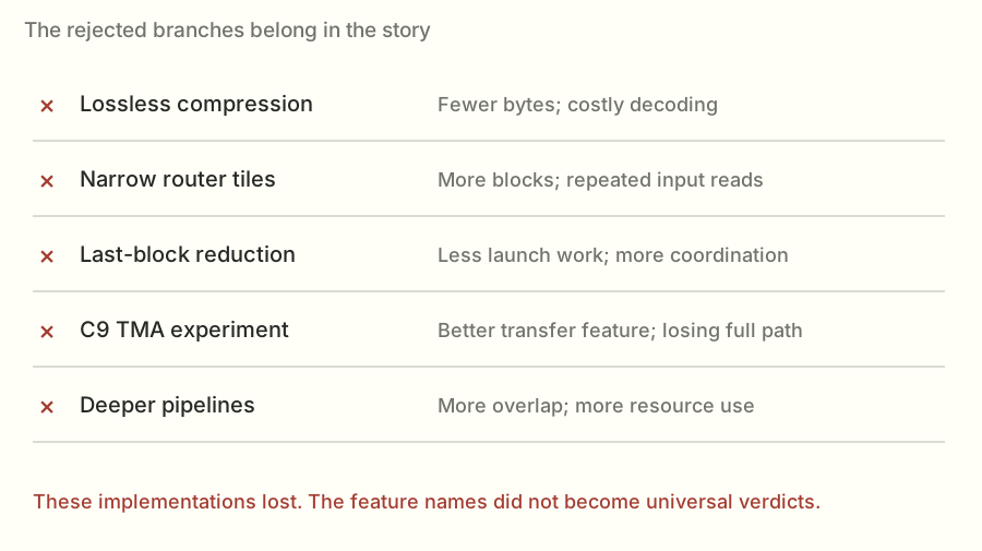
Deeper QKV pipelines and more pooler refinements also failed to produce a clear next improvement. Some choices were obviously worse; others were close enough that I didn't want to replace a working setting on the strength of one flattering replay.
I kept these failures in the notes. They mattered later, especially because a different TMA design eventually did help. “I tried this feature once” isn't the same as having tested every way to use it.
The change that finally took me over 1.30×#
After all that, the next useful improvement came from revisiting the one-token vector path.
At one token, there isn't much reuse of a weight across token rows. The kernel reads the input vector, reads the weights, multiplies, and sums. The C10 search revisited how many output rows each block owned, how many warps it used, and how it treated the weight stream in cache.
For the selected QKV and pooler entries, the useful configuration was one output row per block, sixteen warps, and .cg weight loads. The .cg setting controls cache behavior; it lets those weight loads use the global caching path without using L1. The much smaller input vector had different reuse needs, so it received different treatment.
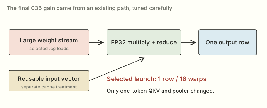
The local paired comparisons repeatedly found useful gains in these one-token cases: roughly six percent for QKV and just under five percent for pooler in a later retest. Those are component improvements in that local comparison, not percentages I could simply add to the overall score.
Read the one-token kernel from addresses to output#
The mathematical job is one dot product per output row. With one output row per program, the grid has N programs. row = program_id(0) * BN + arange(0, BN) identifies the owned output row or rows; the selected BN is one.
col = arange(0, BK) identifies logical K positions. BK is chosen as the next power of two at least as large as K. That makes the reduction structure convenient, and the masks prevent padded positions from contributing when necessary.
The weight address expression is W + row[:,None] * K + col[None,:]. The None entries introduce axes so row indices and K indices broadcast into a rectangular index table. “Broadcast” here means apply one index along several logical entries, not physically copy the weight array first.
The input address is X + col, because this path has just one token row. The code converts loaded values to FP32, multiplies matching positions, and uses tl.sum(..., axis=1) to reduce across K. Finally it stores the valid output row, with the required result dtype supplied by the output allocation.
This is the same mathematical dot product from the start of the article. The new details are addresses, masks, formats, and which program owns each sum.
What changing the warp count could change#
Sixteen warps contain 512 threads. For a K of 8,192, an ideal even division would assign about sixteen logical K values per thread. Eight warps would average thirty-two. This is a useful count to build intuition; the compiler's actual mapping and generated instructions determine the real execution.
Changing the warp count can change values held per thread, register allocation, the reduction tree, synchronization, and which blocks can reside together. A larger launch is not simply the old launch with a guaranteed proportional speed increase.
That is why thirty-two warps was a meaningful follow-up test and its regression was meaningful evidence. The measured fact is that the complete 038 candidate checked worse. Without the unavailable counters, I can't assign every part of that loss to one resource limit.
The input and weights had different reuse needs#
At one token, the large weight rows are streamed for their outputs. The small input vector is reused across many output rows. Treating those streams identically in cache isn't automatically optimal.
The selected .cg weight-load setting used the global caching path without L1 caching for those loads. The code kept separate eviction treatment for the input vector. A cache policy is a hardware/compiler instruction choice with constraints; unsupported attribute combinations can fail before there is a valid performance result.
The chosen policy and sixteen-warp launch repeatedly helped the selected one-token QKV and pooler cases locally. The final complete candidate was then checked and scored officially. That last step matters: a tidy explanation of why a cache choice might help does not substitute for the result showing that the bundled source actually did.
The short kernel behind that change
@triton.jit
def _c10_vector(X, W, Y, N: tl.constexpr, K: tl.constexpr,
                 BN: tl.constexpr, BK: tl.constexpr, CACHE: tl.constexpr):
    row = tl.program_id(0) * BN + tl.arange(0, BN)
    col = tl.arange(0, BK)
    if CACHE == '':
        w = tl.load(W + row[:, None] * K + col[None, :],
                    (row[:, None] < N) & (col[None, :] < K), other=0,
                    eviction_policy='evict_first').to(tl.float32)
    else:
        w = tl.load(W + row[:, None] * K + col[None, :],
                    (row[:, None] < N) & (col[None, :] < K), other=0,
                    cache_modifier=CACHE).to(tl.float32)
    x = tl.load(X + col, col < K, other=0, eviction_policy='evict_last').to(tl.float32)
    value = tl.sum(w * x[None, :], axis=1)
    tl.store(Y + row, value, row < N)
Candidate 036 combined those two updated entries with the useful packing, cluster, router, tiny-matrix, and library routes from the earlier work.
The official check passed at 1.3020×. The scored submission passed at 1.3012×.
That was the 1.30× milestone I had been asking for.
The final program wasn't one heroic replacement for matrix multiplication. It was a set of fairly specific choices about which method should run where.
What actually ran in the winning version?#
At one token, QKV and pooler used the new vector path. Small-token QKV used the earlier cooperating-block kernel. Small-token pooler used its packed weights. Other ranges used the selected library orientations or existing library calls. The router used a direct FP32 path at one token and high/low contributions with atomic accumulation above it.
You can inspect those choices here. Change the token count and watch the selected method change:
036’s first matching plan entry. Swapped-output library routes can fall back for M not divisible by eight; applicability guards and full fallback code remain in the linked source.
The exact dispatch entries
PLAN['qkv_gate'] = [(1, 'vector', (1,4)), (16, 'cluster', (8,3,2,128)), (32, 'c7lt', (3,8)), (1<<30, 'cublas', ())]
PLAN['pooler'] = [(1, 'vector', (1,8)), (16, 'c2packed', (16,32,512,2,4)), (32, 'c2packed', (32,32,512,2,3)), (64, 'trans', ()), (128, 'c7lt', (3,1)), (1<<30, 'c7lt', (0,3))]
PLAN['unpooler'] = [(1, 'vector', (1,8)), (8, 'flashinfer', ('tinygemm',)), (128, 'trans', ()), (1<<30, 'c7lt', (3,0))]
The final two lines replace QKV and pooler’s first entries with (1, 'c10vector', (1, 16, '.cg')). Full applicability and fallback logic stays in the exact source.
If you want to see where the time went, here's a more useful picture than the final score alone. These are the saved official 036 timings. Each group shows baseline and candidate times for one load. Lower is better.
Official 036 timings · baseline versus my version · microseconds (μs) · lower is better
Some shapes improved a lot. A few were slightly worse. The full score came from all of them together.
Inspect all thirty official shape timings
| Load | Layer | M / N / K | Baseline μs | 036 μs | Ratio |
|---|---|---|---|---|---|
| decode 1 | qkv_gate | 1 / 2,304 / 8,192 | 14.080 | 10.077 | 1.397× |
| decode 1 | o | 1 / 8,192 / 1,024 | 6.784 | 5.490 | 1.236× |
| decode 1 | pooler | 1 / 4,096 / 8,192 | 21.456 | 16.532 | 1.298× |
| decode 1 | unpooler | 1 / 1,024 / 4,096 | 6.912 | 3.666 | 1.886× |
| decode 1 | router | 1 / 256 / 8,192 | 10.528 | 3.770 | 2.792× |
| decode 16 | qkv_gate | 16 / 2,304 / 8,192 | 14.128 | 12.971 | 1.089× |
| decode 16 | o | 16 / 8,192 / 1,024 | 6.656 | 6.700 | 0.993× |
| decode 16 | pooler | 16 / 4,096 / 8,192 | 21.104 | 18.073 | 1.168× |
| decode 16 | unpooler | 16 / 8,192 / 4,096 | 18.624 | 18.126 | 1.027× |
| decode 16 | router | 16 / 256 / 8,192 | 14.720 | 5.102 | 2.885× |
| decode 32 | qkv_gate | 32 / 2,304 / 8,192 | 14.144 | 13.028 | 1.086× |
| decode 32 | o | 32 / 8,192 / 1,024 | 6.784 | 6.665 | 1.018× |
| decode 32 | pooler | 32 / 4,096 / 8,192 | 21.952 | 18.839 | 1.165× |
| decode 32 | unpooler | 32 / 8,192 / 4,096 | 18.560 | 17.887 | 1.038× |
| decode 32 | router | 32 / 256 / 8,192 | 15.280 | 5.726 | 2.669× |
| verify 1 | qkv_gate | 8 / 2,304 / 8,192 | 13.984 | 12.594 | 1.110× |
| verify 1 | o | 8 / 8,192 / 1,024 | 6.464 | 6.544 | 0.988× |
| verify 1 | pooler | 8 / 4,096 / 8,192 | 21.248 | 18.066 | 1.176× |
| verify 1 | unpooler | 8 / 1,024 / 4,096 | 6.848 | 4.766 | 1.437× |
| verify 1 | router | 8 / 256 / 8,192 | 25.984 | 5.035 | 5.160× |
| verify 16 | qkv_gate | 128 / 2,304 / 8,192 | 17.232 | 17.089 | 1.008× |
| verify 16 | o | 128 / 8,192 / 1,024 | 7.424 | 7.651 | 0.970× |
| verify 16 | pooler | 128 / 4,096 / 8,192 | 24.928 | 21.066 | 1.183× |
| verify 16 | unpooler | 128 / 8,192 / 4,096 | 19.584 | 18.928 | 1.035× |
| verify 16 | router | 128 / 256 / 8,192 | 16.160 | 6.829 | 2.367× |
| verify 32 | qkv_gate | 256 / 2,304 / 8,192 | 20.000 | 19.936 | 1.003× |
| verify 32 | o | 256 / 8,192 / 1,024 | 9.152 | 9.488 | 0.965× |
| verify 32 | pooler | 256 / 4,096 / 8,192 | 30.896 | 28.949 | 1.067× |
| verify 32 | unpooler | 256 / 8,192 / 4,096 | 23.984 | 23.861 | 1.005× |
| verify 32 | router | 256 / 256 / 8,192 | 17.568 | 8.884 | 1.977× |
Download the shape data as CSV. Ratios shown here divide displayed shape estimates; the official aggregate retains the evaluator’s paired-ratio method.
I saved the exact source and official results rather than just keeping a file named “best.” That's how I could come back later and know which program had actually earned the number. They're linked in the code and results page.
The annoying bit: my local run said 1.3234×#
The complete 036 bundle looked encouraging in the lab. It measured about 1.0241× against the saved 033 version, and about 1.3234× against the local SGLang baseline.
By then my target had moved to 1.32×. So the local number looked like I might already be there.
The official result was 1.3012×.
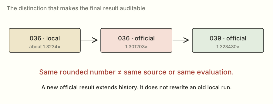
The local setup matched important parts of the judge, but it wasn't identical. Machine and driver details, exact baseline behavior, overhead estimates, and ordinary variation could all contribute. I didn't have an experiment that proved one cause explained the whole gap.
So I kept the local number labeled local and used the official result for the achievement. The local run had helped me choose what to submit. It didn't get to decide what the competition recorded.
A couple of follow-ups made the point even clearer. Candidate 037 removed unused preparation and checked near the previous result, at 1.3022×. Candidate 038 tried thirty-two warps in the selected vector launches and fell back to 1.2699×. More warps hadn't continued the earlier improvement.
To get from 036's official point estimate to 1.32×, I still needed about 1.424% less aggregate time. Small enough to sound easy. Large enough that several plausible ideas hadn't done it.
Percentages are a poor way to choose an isolated winner#
Suppose a load originally spends 40 μs in one component and 10 μs in another. Making the first component 10% shorter saves 4 μs. Making the second 20% shorter saves 2 μs. The smaller percentage saved more total time because it acted on the larger component.
The updated load times would be 46 μs for the first change and 48 μs for the second. Their speedups over the original 50 μs are about 1.0870× and 1.0417×. That's why I looked at actual time shares rather than ranking individual percentage gains.
Now include the six-load geometric mean. If only one load gains a factor r and the others stay unchanged, the overall relative factor is r^(1/6). A 6% improvement in one load's speed ratio is only about a 0.98% overall relative improvement. A win in one shape is diluted further if the shape is only part of that load.
The logarithm form of the formula is the same calculation in different notation. The natural logarithm, written log or ln here, turns multiplication into addition: ln(a×b) = ln(a) + ln(b). Its inverse, exp, turns the result back. So averaging six log ratios and applying exp is equivalent to multiplying six positive ratios and taking the sixth root. The logarithm isn't an extra scoring penalty; it is a convenient way to express the geometric mean.
That doesn't make small gains useless. It tells me how many useful pieces I may need and what a proposed experiment can plausibly contribute to the target.
Derive the remaining 1.32× gap#
Take the officially scored 036 point estimate, about 1.301203×. To reach a score of 1.32× with the same baseline, the required relative speed factor is 1.32 / 1.301203, about 1.01445. The required time fraction is its reciprocal, about 0.98576. So I need about 1.424% less aggregate time.
If only one of the six load ratios changed, its required relative speed factor would be approximately 1.01445^6, about 1.09. That's roughly nine percent faster in that load, and the corresponding percentage time reduction is a little smaller. If I only improve one component within the load, it needs enough time share to produce that load-level gain.
This was planning arithmetic. It did not mean that finding a noisy 1.424% local improvement would guarantee an official target crossing. The later result had to come from another passing official evaluation.
Why a projection score isn't a serving promise#
Let f be the fraction of a system's original time spent in the part I accelerate, and s its speedup. The unchanged part takes 1−f of the old time. The accelerated part now takes f/s. The total normalized time is (1−f)+f/s, so total speedup is the reciprocal.
If a component accounted for 20% of the original time and became infinitely fast, the other 80% would still remain. The maximum total speedup would be 1/0.8 = 1.25×. If that component merely doubled in speed, total time becomes 0.9 and speedup is about 1.1111×.
For serving, I also have to care about latency, the time a person waits, and throughput, how much work the system finishes per unit time. Larger batches can improve reuse and throughput while making a lightly loaded request wait longer for a batch. Kernel improvements can help those tradeoffs, but a component score alone doesn't measure their final effect.
The practical next test would integrate the exact verified source where its shapes and contracts match, then measure full-system behavior. That includes time to the first token, time between later tokens, tokens per second, communication, and scheduling. The article's 1.3234× remains the projection benchmark result I actually have.
The later version really did reach 1.32×#
Candidate 039 eventually checked at 1.3218× and independently scored 1.3234×. The saved leaderboard read had it at 66th out of 796 ranked entries on October 24, 2026.
This is a different result from that earlier local 1.3234×. Different code, different evaluation. The matching rounded number is just a slightly confusing coincidence.
Three additions went into the later version. The first was about when to wait.
The atomic router still needed a zero-filled output. But it could load inputs and calculate products before it was ready to add to that output. The new path used programmatic dependent launch, or PDL, to give that independent work an opportunity to begin early, then waited before the output writes that needed initialization to be finished.
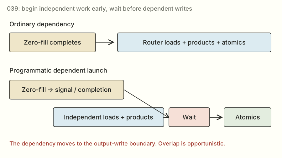
An everyday version: I can start chopping ingredients while water heats up. I still have to wait for the water before doing the step that needs boiling water. Moving the wait doesn't remove the dependency. On the GPU, the overlap is opportunistic, so the code also has to work if the hoped-for overlap doesn't happen.
The exact dependency I was trying to shorten#
For the atomic router, zero-fill produces initialized output memory. The following router kernel consumes inputs and weights to calculate a partial, then adds that partial into the output. The loads and product computation don't depend on the new output values; the atomic update does.
A normal same-stream dependency waits for the predecessor before starting the next kernel's work. With programmatic dependent launch, the implementation can signal that the following kernel may begin independent work earlier. The consumer then performs the required dependency wait before the point where the predecessor's results are needed.
This is a dependency-graph idea: preserve the edge at the operation that needs it instead of treating the entire following kernel as dependent from its first instruction.
The savings, if any, come from execution overlap or hidden launch latency. The memory initialization still happens, every partial still contributes, and the correctness order at the output boundary is preserved.
What the wait must not become#
The implementation cannot rely on the GPU guaranteeing that both kernels run concurrently. NVIDIA describes this opportunity as opportunistic. A design that needs a consumer to run simultaneously for the producer ever to finish can deadlock if the scheduling doesn't provide that overlap.
The saved source signals dependent launch and waits at the dependent-write boundary. The official passing result is evidence for the evaluated source. The scheduling mechanism's meaning comes from the CUDA PDL documentation; the box widths in my drawing are only illustrative.
This is also why I'd avoid describing the later router as having removed initialization. It reorganized when work could begin relative to initialization. Removing a dependency and postponing a wait are different changes, with different correctness obligations.
The second addition was more specific cuBLASLt choices for QKV at 128 tokens and pooler at 256. The nearby sizes kept earlier routes. An algorithm index in one of these searches identifies a choice in that shape's list; it isn't a magic number that I can apply to every matrix.
The third was a new skinny QKV design for the selected 9–32-token range. “Skinny” describes the relatively small token dimension. This version used TMA to move tiles and WGMMA, or warp-group matrix multiply-accumulate, for cooperative matrix arithmetic. It organized producer work, consumer work, staging buffers, and cluster reduction together.
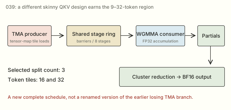
The selected configurations used three-way split work and an eight-stage pipeline, with token tiles of 16 and 32. This was a different complete implementation from both the earlier losing TMA branch and the earlier cp.async / mma.sync kernel.
That's why keeping the failed branch mattered. The lesson from it was that a particular implementation lost. A later design still deserved to be measured.
The scored result's reported interval was about 1.3036× to 1.3433×. That interval describes uncertainty in the measurement; it isn't a promise that every future run will land inside it. The passing official point estimate crossed the 1.32× target. It didn't give me a guarantee that every repeat would beat 1.32×, or tell me the exact isolated contribution of each addition.
The original 1.301203× scored run is d296d0c1b1774e5e. The later 1.323430× scored run is f7219946bf314f37. The code and results page includes the exact source files, their hashes, and both later check and scored results.The two milestones, with exact result files
Everything I tried, if you want to poke around#
Here's the full saved evaluation log. You can search by candidate number, method name, problem, or job ID. A candidate is just a numbered version of the program I tested. A job is one evaluation of it.
Some versions have both a check and a scored run. Some failed. Candidate 030's separate check was still queued in this saved log even though its scored submission had finished. A dash means there wasn't a usable speedup for that row.
| Candidate | Problem / mode | Outcome | Ratio / reported interval | Job evidence |
|---|---|---|---|---|
| 001 first-candidate | muse_bf16_proj check | PASS | 0.776071×[0.7644, 0.7877] | f866e678b7224915 |
| 002 split-router | muse_bf16_proj check | PASS | 1.101364×[1.0848, 1.1179] | 572e74a3ffab41c5 |
| 003 selective-gemv | muse_bf16_proj check | PASS | 1.012148×[0.9970, 1.0273] | f4d0168f5de64fb5 |
| 004 router-dispatch | muse_bf16_proj check | PASS | 1.116059×[1.0993, 1.1328] | e5af02cdbd7f406c |
| 005 attention-fused-prep | muse_attention_decode check | PASS | 1.132496×[1.1155, 1.1495] | 58b3a19d62ba47e9 |
| 006 moe-local-tiles | muse_moe_w4a16 check | PASS | 0.994488×[0.9796, 1.0094] | 70a33e31fcff4209 |
| 007 dense-splitk | muse_bf16_proj check | PASS | 1.049125×[1.0334, 1.0649] | 5b873c781e7142e4 |
| 002 split-router | muse_bf16_proj scored | PASS | 1.103685×[1.0871, 1.1202] | cc6781ae999346d3 |
| 009 packed-router | muse_bf16_proj check | PASS | 1.137166×[1.1201, 1.1542] | 50425507196b4c28 |
| 004 router-dispatch | muse_bf16_proj scored | PASS | 1.114445×[1.0977, 1.1312] | 5a243a8bf9374769 |
| 010 moe-fused-postnorm | muse_moe_w4a16 check | PASS | 1.147244×[1.1300, 1.1645] | 04da63a66c674637 |
| 005 attention-fused-prep | muse_attention_decode scored | PASS | 1.132288×[1.1153, 1.1493] | 87e5773111914b12 |
| 009 packed-router | muse_bf16_proj scored | PASS | 1.155506×[1.1382, 1.1728] | 1eb88f402c9e49ff |
| 010 moe-fused-postnorm | muse_moe_w4a16 scored | PASS | 1.145379×[1.1282, 1.1626] | c0212e53511a4f5f |
| 011 layer-validated-components | muse_decode_layer check | PASS | 1.093329×[1.0769, 1.1097] | 913fa5827cea45ee |
| 012 attention-local-splits | muse_attention_decode check | PASS | 1.134850×[1.1178, 1.1519] | a7a822fec0c2496c |
| 013 moe-middle-tiles | muse_moe_w4a16 check | PASS | 1.270556×[1.2515, 1.2896] | 893eaf3246294d11 |
| 014 hopper-gemv | muse_bf16_proj check | PASS | 1.148147×[1.1309, 1.1654] | 943a9df9c1c04687 |
| 015 transposed-dense | muse_bf16_proj check | PASS | 1.167969×[1.1504, 1.1855] | cc943620312d4c31 |
| 016 wide-k-dense | muse_bf16_proj check | PASS | 1.135331×[1.1183, 1.1524] | 701cf501581641c8 |
| 017 quack-large-dense | muse_bf16_proj check | FAILED | — | 9f4513b067514f58 |
| 018 quack-skinny-swapped | muse_bf16_proj check | FAILED | — | 5e333e121f334aab |
| 019 quack-large-batched | muse_bf16_proj check | PASS | 1.000884×[0.9859, 1.0159] | aced8156133042c4 |
| 020 quack-skinny-batched | muse_bf16_proj check | PASS | 1.122068×[1.1052, 1.1389] | d40938c864f642d1 |
| 013 moe-middle-tiles | muse_moe_w4a16 scored | PASS | 1.268370×[1.2493, 1.2874] | 95d955a276954ab1 |
| 011 layer-validated-components | muse_decode_layer scored | PASS | 1.095338×[1.0789, 1.1118] | 8b390705f33c4de4 |
| 022 cublaslt-plan-search | muse_bf16_proj check | PASS | 1.159035×[1.1416, 1.1764] | 5abcfb3369c54def |
| 023 vector-plan-search | muse_bf16_proj check | PASS | 1.181509×[1.1638, 1.1992] | 5015611a0b174a37 |
| 024 router-plan-search | muse_bf16_proj check | PASS | 1.142180×[1.1250, 1.1593] | 65ed6dcb8e854027 |
| 021 measured-dense-bundle-ca23de4a9240 | muse_bf16_proj check | PASS | 1.162327×[1.1449, 1.1798] | d31d8309a7b2493f |
| 025 router-single-launch | muse_bf16_proj check | PASS | 1.142189×[1.1251, 1.1593] | e8478220d206462e |
| 027 paired-router-search | muse_bf16_proj check | PASS | 1.153926×[1.1366, 1.1712] | af4bdc2fdc3d4e9f |
| 028 cublaslt-expanded-search | muse_bf16_proj check | PASS | 1.178338×[1.1607, 1.1960] | 44171a897181430a |
| 026 expanded-bundle-c0f93b5a0027 | muse_bf16_proj check | PASS | 1.209900×[1.1918, 1.2280] | 16196285af6f4000 |
| 026 expanded-bundle-c0f93b5a0027 | muse_bf16_proj scored | PASS | 1.199334×[1.1813, 1.2173] | eb6210fc448642f8 |
| 029 c1-bestof | muse_bf16_proj check | PASS | 1.256396×[1.2375, 1.2752] | f047171bd8e24058 |
| 030 c1-atomic-router | muse_bf16_proj check | QUEUED | — | d348735a9f334e7a |
| 030 c1-atomic-router | muse_bf16_proj scored | PASS | 1.278497×[1.2593, 1.2977] | f532c7ddea4149a4 |
| 031 c1-tinygemm-unpooler | muse_bf16_proj check | PASS | 1.261956×[1.2430, 1.2809] | 30305751fd10410b |
| 032 c1-cluster-qkv | muse_bf16_proj check | PASS | 1.271215×[1.2521, 1.2903] | 228a4d9dcc8c46b9 |
| 033 c1-deep-cluster-qkv | muse_bf16_proj check | PASS | 1.277069×[1.2579, 1.2962] | e22801f8d913429f |
| 033 c1-deep-cluster-qkv | muse_bf16_proj scored | PASS | 1.288792×[1.2695, 1.3081] | 54eb1a07e4014863 |
| 034 c2-packed-cublaslt | muse_bf16_proj check | PASS | 1.285194×[1.2659, 1.3045] | 769082fea33045cc |
| 035 c2-pooler-lt-layouts | muse_bf16_proj check | PASS | 1.286016×[1.2667, 1.3053] | 0ca0f57f661247b0 |
| 036 c2-streaming-vector | muse_bf16_proj check | PASS | 1.302007×[1.2825, 1.3215] | e8442a3e94034bb4 |
| 036 c2-streaming-vector | muse_bf16_proj scored | PASS | 1.301203×[1.2817, 1.3207] | d296d0c1b1774e5e |
| 037 c2-lean-preparation | muse_bf16_proj check | PASS | 1.302160×[1.2826, 1.3217] | d4a592817b414146 |
| 038 c2-vector32 | muse_bf16_proj check | PASS | 1.269896×[1.2508, 1.2889] | d5322fc0e8e44207 |
| 039 c20-pdl-router-lt15-skinny | muse_bf16_proj check | PASS | 1.321790×[1.3020, 1.3416] | 17f2e7a210cd4fcd |
| 039 c20-pdl-router-lt15-skinny | muse_bf16_proj scored | PASS | 1.323430×[1.3036, 1.3433] | f7219946bf314f37 |
The ledger contains 50 evaluation records. “—” means no usable speedup was established for that row. Download JSON.
The log covers the preserved 001–038 results plus 039's later check and submission. The longer experiment notes also cover source-only branches. Having a source file is different from having a completed, passing result for it.
What I took away from all this#
I started by asking for a number. Getting to it meant learning to ask smaller questions.
Am I giving the GPU enough independent work? Am I fetching the same values more often than I need to? Is a layout making an otherwise good library call awkward? Does the thing I removed cost less than the thing I added? Am I even measuring the same conditions as the judge?
The answers changed as the program improved. Splitting a sum helped when the output grid was small. Combining partials differently helped later. Packing weights and choosing library orientations helped particular sizes. Revisiting a one-token kernel helped after several more elaborate attempts had lost.
I also got more careful about what a measurement actually established. A correct answer wasn't automatically fast. A good local timing wasn't automatically an official score. A faster component wasn't automatically a faster complete submission. And a newer source file wasn't automatically the new best.
The result I can point to is 1.3234× on the dense-projection benchmark, with the earlier 1.3012× milestone preserved too. The more useful thing I got out of it is a trail I can follow: here's the problem, here's what I tried, here's the result, and here's why I kept going in that direction.
If you've made it this far without knowing GPU programming beforehand, the next layer of detail is below. It covers the model, the math, all thirty shapes, the source walkthrough, the failed experiments, and a glossary. Read it in order, or search for the bit you're curious about.
- 01 The run that crossed 1.30×
- 02 What the competition actually asks
- 03 The complete competition map
- 04 From a message to generated tokens
- 05 Inside the transformer layer
- 06 Prefill, decode, and verification
- 07 One GPU inside an eight-GPU model
- 08 The software stack beneath SGLang
- 09 The mathematics of our projection
- 10 The exact projection workload
- 11 Numerical formats and error
- 12 Why the router needs special care
- 13 A guided tour of the H200
- 14 Threads, warps, blocks, and scheduling
- 15 The journey of a byte
- 16 Coalescing, tiling, and weight layout
- 17 Tensor cores and matrix instructions
- 18 Rooflines and practical limits
- 19 Split-K and the cost of combining work
- 20 Hopper pipelines and block clusters
- 21 The submission contract
- 22 What correctness really tests
- 23 How the judge times a kernel
- 24 How thirty timings become one score
- 25 Noise, uncertainty, and moving ranks
- 26 Building an auditable investigation
- 27 A correct kernel that lost
- 28 Split the router: our first useful win
- 29 Learning to dispatch by shape
- 30 Packed router: reaching 1.1555×
- 31 The attention side story
- 32 The routed-expert side story
- 33 Why whole-layer gains were smaller
- 34 Transposes, wider K, and QuACK detours
- 35 Systematic vector and library searches
- 36 Composing gains into 1.1993×
- 37 The handoff and the measured best-of plan
- 38 Atomic router: reaching 1.2785×
- 39 The small unpooler opportunity
- 40 Custom cluster QKV: reaching 1.2888×
- 41 Building our remote H200 laboratory
- 42 The packed pooler experiment
- 43 Exploring cuBLASLt orientations
- 44 Lossless compression: fewer bytes, slower execution
- 45 Router redesigns that did not help
- 46 Advanced features that still lost
- 47 The final single-token streaming gain
- 48 Read the winning implementation end to end
- 49 Local 1.3234×, official 1.3012×
- 50 What crossing 1.30× established
- 51 The epilogue: tuning can regress
- 52 The remaining road to 1.32×
- 53 From kernel wins to serving wins
- 54 Reproduce and audit the result
- 55 The decision-making playbook
- 56 Appendix A · Every experiment
- 57 Appendix B · All thirty shapes
- 58 Appendix C · Mathematical derivations
- 59 Appendix D · The source atlas
- 60 Appendix E · The glossary
- 61 Appendix F · Provenance and limitations
- 62 Appendix G · Pause and predict
- 63 Postscript · The official 1.3234× result
No matching chapter. Try another term.
Code, results, and things I found useful#
The code and results page has the saved sources, official evaluations, and downloadable data. The thirty-shape CSV is useful if you want to do your own timing breakdown. The exact winner files are preserved so you can check what earned each score.
For competition details, there's the Open Kernel Challenge and its rules. The archived schedule in my notes closed the kernel stage on November 4, 2026, at 11:59 p.m. Pacific and started serving on November 5 at noon. The schedule and leaderboard in this article are dated snapshots.
The format of this post owes a lot to Simon Boehm's CUDA matrix-multiplication worklog. I liked how it made room for intermediate versions and explained why each next step was worth trying. That's the kind of article I wanted this to be.
If you want to go further into the implementation, the Hopper tuning guide, cuBLAS/cuBLASLt reference, Triton matrix-multiplication tutorial, and PDL documentation are the deeper references. You don't need to read them before understanding the story above.