# How I made Muse’s GPU projections 1.32× faster in the Open Kernel Challenge

## This started with a fairly simple question

“Can we get at least 1.3×?”

That was the goal. There was a competition called the Open Kernel Challenge, people were posting speedups over an existing implementation, and I wanted to see how far I could get.

The first version I tested came back at **0.7761×**.

If you're wondering whether that's good: no. One means I matched the starting point. Below one means I made it slower. The code gave the right answers, but it took longer to get them.

So this became a story about figuring out what “faster” actually requires. Sometimes I needed more work running at once. Sometimes I needed to move the same numbers into a different arrangement. Sometimes the best move was to keep using an existing library. And quite a few things that sounded clever just lost.

I eventually got an official **1.30×**, then **1.3234×**, on the part of the model I was working on. I'll explain what that means in a bit. It doesn't mean the entire AI model suddenly got 32% faster.

I worked with Claude and Codex along the way. This is my walkthrough of that process: what I tried, what the results said, and what I kept. I'm going to build the math and the GPU concepts from the ground up, then use them to explain the real experiments. No linear algebra or CUDA background assumed. The point is to understand the work well enough that the next design choice makes sense.

This is a long read. I use small numerical examples first, then connect them to the actual source and timings. When I say an example is illustrative, its numbers explain a concept; the experiment tables are the recorded results. You can leave and come back using the section links below the title.

## Okay, what is the model doing in the first place?

When you send a message to a language model, it turns the text into **tokens**. A token is a small piece of text: sometimes a word, sometimes part of a word, sometimes punctuation. The model represents those tokens as lists of numbers and runs calculations on them to predict what should come next.

A lot of those calculations are variations of the same thing: take some input numbers, multiply them by some stored numbers, and add the results.

Those stored numbers are called **weights**. Training chooses the weights. When I'm running the model to answer a message, the weights are already there; I'm using them to transform the input. That answering stage is called **inference**.

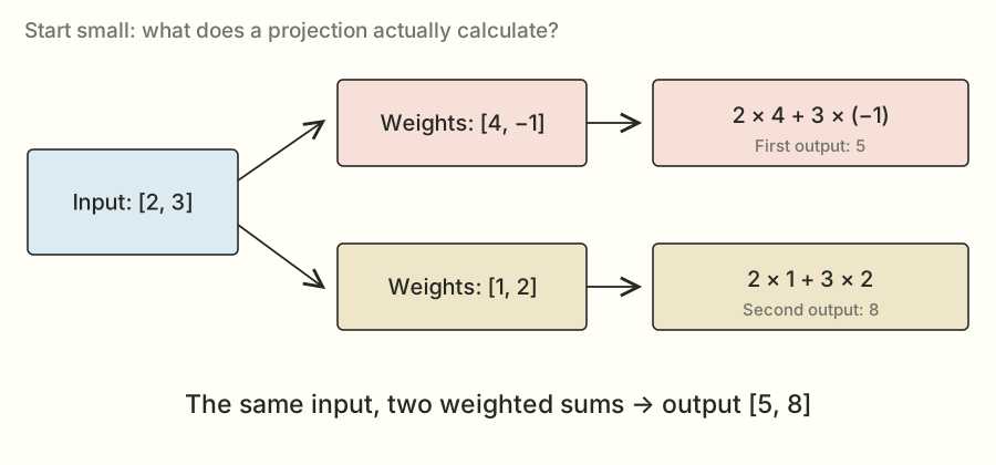
Here's a deliberately tiny example. Say the input is `[2, 3]`, and one set of weights is `[4, -1]`. Multiply matching entries, then add them:

<div class="equation">2 × 4 + 3 × (−1) = 5</div>

A different set of weights, `[1, 2]`, gives `2 × 1 + 3 × 2 = 8`. So the same input can produce an output list `[5, 8]`. A **dense projection** does this sort of weighted sum over much bigger lists. “Dense” means the calculation uses the full matrix of weights rather than a selected sparse subset.

<figure id="fig-tiny" class="wide"><a href="assets/tiny.svg" aria-label="Open full-size diagram: Two weighted sums, drawn out."><img src="assets/tiny.svg" alt="Two weighted sums, drawn out. Each output multiplies the input entries by its own weights, then adds the products. A real projection does this with thousands of entries and output features." loading="lazy" width="900" height="450"></a><figcaption><b>Two weighted sums, drawn out.</b> Each output multiplies the input entries by its own weights, then adds the products. A real projection does this with thousands of entries and output features.</figcaption></figure>

Put lots of input lists and weight lists into rectangular tables, and you get **matrix multiplication**. The tables are matrices. The multiplication is a compact way to ask for all those weighted sums.

The real calculation might use 8,192 input numbers for each token and produce thousands of outputs. Repeat this inside a model, over many tokens, and small differences in how you run the calculation start to matter.

<aside class="sidenote"><b>A matrix is just a table of numbers.</b> The intimidating part is usually the size and the indexing. The basic multiply-and-add operation is still the one in the little example.</aside>

## I'm going to unpack the math properly

The little weighted-sum example is the calculation I kept coming back to. But I want to build the vocabulary around it carefully, because later choices about tiles, reductions, and transposes make much more sense when the math is familiar.

Start with a **scalar**: one number, like `3`. A **vector** is an ordered list of numbers, like `[2, 3]`. A **matrix** is a rectangular arrangement of numbers, like a spreadsheet with a fixed number of rows and columns. A **tensor** is the more general term for an array with some number of dimensions. A scalar, vector, and matrix can be viewed as zero-, one-, and two-dimensional tensors.

Here, “dimension” can mean two related things. The vector `[2, 3]` has two coordinates. A matrix has two axes, rows and columns, but each of those axes can contain thousands of entries. When I say the matrix has **shape [16, 8,192]**, I'm saying it has 16 rows and 8,192 columns. I'm not saying it has only two stored numbers.

The order matters. `[2, 3]` and `[3, 2]` are different vectors. Swapping input features while leaving their weights alone generally changes the answer, just as swapping the quantity and price columns in a spreadsheet would change what a formula means.

### Addition and scaling come first

To add two vectors of the same length, add matching entries. `[2, 3] + [1, -2] = [3, 1]`. To multiply a vector by a scalar, multiply every entry: `4 × [2, 3] = [8, 12]`.

Those operations already explain part of what a projection does. A weight scales how much one input feature contributes to an output. A positive weight contributes in the same sign as the input; a negative weight can subtract. A zero weight contributes nothing to that particular sum.

I don't need to attach a human-readable meaning like “happiness” or “grammar” to each feature. Inside a learned model, the coordinates are learned numerical representations. My kernel's job is to transform the numbers according to the specified weights, regardless of what an individual coordinate might mean.

### A dot product makes one output number

The **dot product** of two equally long vectors multiplies corresponding entries and adds the products:

<div class="equation">[2, 3] · [4, −1] = (2 × 4) + (3 × −1) = 5</div>

The result is one scalar. It isn't the vector `[8, -3]`; that vector would be the **elementwise product** before the final addition. This distinction will matter in the expert block later, where some multiplications really are element by element.

For a longer example, take `[1, -2, 3]` and `[4, 5, -1]`. Their products are `4`, `-10`, and `-3`. Add them and the dot product is `-9`. Negative answers are perfectly ordinary. A linear projection is not a probability calculation by itself.

If you've seen the symbol **Σ** and wondered where the complicated math started, this is all it is doing here: telling me to add a sequence of terms. I can write the same dot product as `Σₖ xₖwₖ`. The little `k` is an index pointing to matching positions in the two lists.

In code I usually start indices at zero. With K input features, the positions are `0, 1, …, K−1`. That gives K positions, just as the floors numbered 0 through 4 give five floors.

### Matrix multiplication is a whole collection of dot products

I'll keep two token rows together in an input matrix X, and use three weight rows in W:

<div class="matrix-example"><div><b>Input X · 2 rows × 2 features</b><pre> 2   3
 1  −2</pre></div><div><b>Weights W · 3 outputs × 2 features</b><pre> 4  −1
 1   2
−2   3</pre></div></div>

For the first token row `[2, 3]`, I take a dot product with **every row of W**. They give `5`, `8`, and `5`. For the second token row `[1, -2]`, the same three weight rows give `6`, `-3`, and `-8`.

The output matrix is therefore:

<div class="equation">Y = [[5, 8, 5], [6, −3, −8]]<small>Two token rows in. Three output features per row out.</small></div>

There are six output cells because there are two tokens and three output features: `2 × 3 = 6`. Every output is a dot product of length two, because every input row and every weight row have two features.

Try selecting an output cell below. The highlighted input row and weight row are the two vectors used for that cell. Move the slider to include zero, one, or both terms of the sum.

<section class="interactive matrix-lab" aria-label="Work through a matrix product"><div class="eyebrow">Calculate one output with me</div><p class="small">Teaching example · exact small integers · no benchmark claims</p><div class="matrix-controls"><label>Token row <select id="matrix-row"><option value="0">0: [2, 3]</option><option value="1">1: [1, −2]</option></select></label><label>Output feature <select id="matrix-col"><option value="0">0: weights [4, −1]</option><option value="1">1: weights [1, 2]</option><option value="2">2: weights [−2, 3]</option></select></label></div><div class="matrix-grid"><div class="lab-matrix"><p>X</p><table id="matrix-x"><tbody><tr><td data-row="0" data-col="0">2</td><td data-row="0" data-col="1">3</td></tr><tr><td data-row="1" data-col="0">1</td><td data-row="1" data-col="1">-2</td></tr></tbody></table></div><div class="lab-matrix"><p>W</p><table id="matrix-w"><tbody><tr><td data-row="0" data-col="0">4</td><td data-row="0" data-col="1">-1</td></tr><tr><td data-row="1" data-col="0">1</td><td data-row="1" data-col="1">2</td></tr><tr><td data-row="2" data-col="0">-2</td><td data-row="2" data-col="1">3</td></tr></tbody></table></div><div class="lab-matrix"><p>Wᵀ</p><table id="matrix-wt"><tbody><tr><td data-row="0" data-col="0">4</td><td data-row="0" data-col="1">1</td><td data-row="0" data-col="2">-2</td></tr><tr><td data-row="1" data-col="0">-1</td><td data-row="1" data-col="1">2</td><td data-row="1" data-col="2">3</td></tr></tbody></table></div><div class="lab-matrix"><p>Y</p><table id="matrix-y"><tbody><tr><td data-row="0" data-col="0">5</td><td data-row="0" data-col="1">8</td><td data-row="0" data-col="2">5</td></tr><tr><td data-row="1" data-col="0">6</td><td data-row="1" data-col="1">-3</td><td data-row="1" data-col="2">-8</td></tr></tbody></table></div></div><label for="matrix-k">Include <output id="matrix-k-label">2</output> of the 2 K terms</label><input id="matrix-k" type="range" min="0" max="2" step="1" value="2"><div id="matrix-equation" class="result" aria-live="polite">Y[0,0] = 2×4 + 3×(−1) = 5</div><p id="matrix-explanation" class="small">X row 0 meets W row 0, which becomes column 0 of Wᵀ.</p></section>

The bottom-right output is a useful one to check by hand. Its input is `[1, -2]`; its weights are `[-2, 3]`. So it is `1 × (-2) + (-2) × 3 = -2 - 6 = -8`. If you can follow that calculation, you can follow the mathematical operation inside the real projection. The GPU version makes the arrays bigger and the execution much more organized.

### Why the transpose appears

The standard rule for matrix multiplication says: **a row of the left matrix meets a column of the right matrix**. I stored each output's weights in a row of W, so I use W's transpose to make those rows appear as columns.

For this example:

<div class="matrix-example"><div><b>W · shape [3, 2]</b><pre> 4  −1
 1   2
−2   3</pre></div><div><b>Wᵀ · shape [2, 3]</b><pre> 4   1  −2
−1   2   3</pre></div></div>

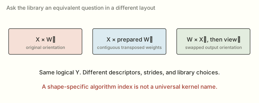
Transposing changes which axis I call rows and which I call columns. It doesn't turn `4` into some new numerical value. Later I'll distinguish viewing an array with different strides from actually copying it into a new contiguous order. Both can describe the same logical transpose while creating different memory-access behavior.

Now the shapes line up:

<div class="equation">[M, K] × [K, N] → [M, N]<br>[2, 2] × [2, 3] → [2, 3]</div>

The **inner dimensions match** because each dot product needs two equally long vectors. The **outer dimensions remain** because I need one result for every input row and every output feature.

This also explains why matrix multiplication usually can't be swapped around. Changing `A × B` to `B × A` changes which rows meet which columns, and sometimes the dimensions don't even permit the swapped product. A library-layout experiment needs an algebraically equivalent transformation, not a casual reordering of the multiplication.

### The full equation, now with the letters explained

For this task, the output cell at token row m and output feature n is:

<div class="equation">Y[m, n] = Σ<sub>k=0…K−1</sub> X[m, k] × W[n, k]</div>

Read it slowly: choose one token row `m`; choose one output `n`; visit every input feature `k`; multiply the input by the matching weight; add those products. That's it. M counts how many token rows I have, N counts how many outputs each needs, and K counts how long each sum is.

Here's the straightforward loop version. It's for understanding the math, not the implementation I submitted:

```python
for m in range(M):
    for n in range(N):
        total = 0
        for k in range(K):
            total += X[m, k] * W[n, k]
        Y[m, n] = total
```

The output cells can be computed independently in exact arithmetic. But the K terms within one cell have to be combined. That difference between **independent output work** and **a reduction into one answer** is the reason split-K will show up in the experiment story.

### What makes it linear?

A transformation T is linear when it preserves addition and scalar multiplication: `T(a + b) = T(a) + T(b)` and `T(ca) = cT(a)`. A fixed matrix multiplication has those properties in exact arithmetic. For example, using the weight row `[4, -1]`, the inputs `[2, 3]` and `[1, -2]` produce `5` and `6`. Add the inputs to get `[3, 1]`, and the output is `12 - 1 = 11`, which is also `5 + 6`.

That doesn't make the entire language model linear. The model also contains nonlinear functions, normalizations, attention probabilities, and selection decisions. If I moved one of those across a matrix product as if every operation commuted, I could change the model.

Some neural-network layers also add a fixed bias vector. A matrix product plus a nonzero fixed bias is an affine map rather than a strictly linear one, because zero no longer maps to zero. The projection equation in this task has no bias term, so the linear-map description applies to its specified mathematical operation.

It also doesn't mean every rearrangement of the sum produces bit-identical computer results. Floating-point arithmetic has finite precision. I'll work through that distinction before the router experiments, because it is one of the easiest ways for an algebraically plausible optimization to be wrong.

### The same transformation as a combination of directions

There's another view of that example which makes reuse easier to see. The input `[2, 3]` can be written as `2×[1, 0] + 3×[0, 1]`. Those two unit-coordinate vectors are called the **standard basis**. They isolate one input feature at a time.

Apply the weight matrix to `[1, 0]` and the output is `[4, 1, -2]`, the first feature's contribution to all outputs. Apply it to `[0, 1]` and the output is `[-1, 2, 3]`. The full result is therefore:

<div class="equation">2 × [4, 1, −2] + 3 × [−1, 2, 3]<br>= [8, 2, −4] + [−3, 6, 9]<br>= [5, 8, 5]</div>

The dot-product view computes one output feature at a time. This combination view computes one input feature's contribution to several outputs. They are the same linear transformation. Different kernels organize tiles and reuse around different parts of that shared structure.

It also explains the sparse probe test later. An input with only one nonzero coordinate isolates a scaled column of the stored weight matrix. The test is using the algebra to inspect which values the implementation really used.

<details class="deep"><summary>Pause and try one</summary><p>Use input <code>[3, 1]</code> and the three weight rows from the example. What are the three outputs?</p><p><b>Answer:</b> <code>[11, 5, -3]</code>. The sums are <code>3×4 + 1×(-1)</code>, <code>3×1 + 1×2</code>, and <code>3×(-2) + 1×3</code>. The output still has three features even though the input has two.</p></details>


## Where the GPU and the competition come in

A GPU is good at doing lots of similar calculations at the same time. That's useful when there are thousands of output sums to compute. But owning a fast GPU doesn't automatically make every program on it fast. The work still needs to be divided up and the numbers still need to get to the places doing the arithmetic.

A **kernel** is a program that runs on the GPU. In this competition, I could replace particular calculations with my own implementation, check that the answers were acceptable, and compare its time against the provided starting implementation.

**CUDA** is NVIDIA's platform for programming its GPUs. **Triton** is a language and compiler that let me write GPU kernels in a Python-like style. I could also call existing libraries, which already contain optimized implementations. A big part of this project was deciding which of those tools fit each job.

That starting point was **SGLang**, a system used to run language models. I'll call it the **baseline** from here on. “I got 1.30×” means my submitted implementation was faster than that baseline under the competition's measurement rules.

The challenge had several places to work: dense projections, attention, routed experts, a whole decode layer, and prefill. Attention lets a token use information from other tokens. Routed experts are groups of model weights where the model selects which groups should process an input. A layer combines these pieces with other operations.

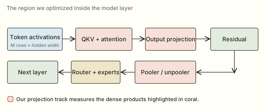
My main story here is the dense-projection problem, named `muse_bf16_proj` in the files. It's one part of Muse Spark Open. Here's where that part sits in the bigger picture:

<figure id="fig-model" class="wide"><a href="assets/model.svg" aria-label="Open full-size diagram: The part of the model I was working on."><img src="assets/model.svg" alt="The part of the model I was working on. The coral boxes are dense projections. Other parts of the layer still take time, which is why a projection speedup is only part of the full-model story. This is a simplified map." loading="lazy" width="900" height="450"></a><figcaption><b>The part of the model I was working on.</b> The coral boxes are dense projections. Other parts of the layer still take time, which is why a projection speedup is only part of the full-model story. This is a simplified map.</figcaption></figure>

The important thing to keep in mind is that improving one box doesn't make every other box faster. If you speed up the engine of a car, you're still going to wait at a red light. In the model, other calculations, communication, and serving overhead still take time.

There's also a full model walkthrough in <a href="notebook.html#chapter-02">my longer notes</a>. I'll connect the main pieces here before narrowing the story to projections.

## How those matrices fit into a language model

I don't want “the model” to remain a mysterious box around the kernels. Here's the path from text to the projection work, without assuming you've studied a transformer before.

A tokenizer maps pieces of text to integer IDs. A token ID is an index into an **embedding table**: a learned table of vectors. Looking up that row gives the model a numerical starting representation for the token. The ID itself is not a ranking of meanings; token 500 is not inherently twice as meaningful as token 250.

Inside a layer, the input representations are called **activations**. The model's weights stay fixed during inference, while the activations depend on the current request and the computations before them. This distinction is why I can prepare a weight layout once but must compute a new answer for each new input.

### Attention: use other tokens' information

Attention forms query, key, and value representations, usually abbreviated Q, K, and V. A query represents what a position is looking for; keys provide something to compare it against; values provide the information to combine. These are useful descriptions of the role of the numbers, not literal English questions written into a vector.

For a small numerical illustration, let a query be `[1, 0]` and two keys be `[2, 1]` and `[0, 3]`. Their dot products are `2` and `0`. An actual attention implementation applies its specified scaling and masking before converting eligible scores into weights. Here I'll treat `2` and `0` as already-scaled illustrative scores.

**Softmax** converts scores into positive weights that sum to one. It exponentiates each score and divides by the sum of the exponentials. To make the arithmetic more stable, I can first subtract the largest score from every score. This leaves the normalized result unchanged in exact arithmetic because it multiplies every exponential by the same factor, which cancels in the division.

The exponential is written `eᵗ`, where e is about 2.71828. At zero it is one; at negative two it is `1/e²`, about 0.1353. It turns these scores into positive numbers before the normalization. Softmax isn't just dividing the original scores by their sum: original scores can be negative, and their sum can be zero.

For scores `[2, 0]`, subtracting 2 gives `[0, -2]`. The exponentials are about `[1, 0.1353]`, so the normalized weights are about `[0.8808, 0.1192]`. If the two value vectors are `[10, 0]` and `[0, 20]`, their attention-weighted sum is about `[8.808, 2.384]`.

That example shows three different operations: dot products make scores; a nonlinear normalization makes probabilities; a weighted sum combines values. My dense QKV projection helps create the Q, K, and V representations. It isn't the entire attention calculation.

The **K in “key”** and the **K in the GEMM dimension** are two uses of the same letter. In the projection equation, K always means the input/reduction width. Context decides which meaning is intended.

### Masks and the key/value cache

When generating text, a token must not use information from future tokens. A **causal mask** excludes those future positions from its attention. Sliding attention also limits which past positions are eligible. These are part of the required computation, not optional speed tricks.

Previously computed keys and values can be stored in a **KV cache** and reused on later generation steps. That avoids recomputing the old token representations for every new token. A paged cache adds a table mapping logical sequence positions to physical memory locations, so the kernel must preserve both the numerical values and the addressing rules.

This is also why speculative verification is more than “a bigger batch.” When checking several proposed tokens, each query has its own allowed history and prefix. An implementation can't casually let the first new query read later proposed tokens.

### Experts: another use of matrix products

A mixture-of-experts block uses router scores to choose a subset of expert networks for a token. The selected expert computations still contain matrix products. They also contain nonlinear operations and, in this task, specified normalization and weighting steps.

One common pattern produces a gate vector and an up vector, transforms the gate with a nonlinear function, multiplies the two vectors elementwise, then applies another matrix product. Notice that **elementwise multiplication** has returned: each gate entry multiplies the corresponding up entry. It does not sum all the features into one dot product at that point.

The nonlinear function means I can't generally push that elementwise work through a matrix multiplication as if everything were one linear map. Fusing operations is useful only if their dependencies and numerical meaning survive.

The routed-expert track used its own weight representation and rules. My dense-projection track preserved its original BF16 dense weights and the allowed router scheme. A technique allowed for a quantized expert problem doesn't automatically become a legal dense-weight approximation.

### Normalization and residuals also cost time

**RMS normalization** computes a scale from the mean of squared features in a row, with a small specified epsilon for stability, then rescales the row. For `[3, 4]`, the mean square is `(9 + 16)/2 = 12.5`, and its square root is about `3.5355`. Ignoring epsilon and learned scaling just for this illustration, dividing by that gives about `[0.8485, 1.1314]`.

That is different from subtracting the average of the row. The operation's exact position matters too: normalizing individual expert outputs before combining them generally differs from normalizing their combined sum.

A **residual connection** adds an earlier representation back to a transformed representation. Elementwise addition looks cheap beside a large matrix product, but reading and writing the arrays still takes time. When the matrix products become faster, surrounding operations can become a larger fraction of the remaining total.

### Prefill, decode, and running across GPUs

**Prefill** processes the prompt and sets up information used by later generation. **Decode** repeatedly produces the next token. Prefill often supplies many token rows for a matrix product. A lightly batched decode step may supply very few. That's one reason an implementation that likes large matrix products can be awkward for decode.

The full model also uses **tensor parallelism** across GPUs. For a row-partitioned weight matrix, a GPU can compute a subset of output features. For a split input/reduction dimension, GPUs may instead produce partial contributions that need combining. The exact partition is specified by the model and task.

Our projection shapes are the local shapes supplied under that partition. A thread-block cluster inside one H200 is not the same thing as eight GPUs cooperating across the node. I'll use “cluster” for the on-GPU block cooperation in the kernel story; the full serving system has a larger communication problem around it.

That is enough of the surrounding model to see the stakes. A projection kernel is a repeated numerical building block. It needs to deliver the right numbers to the next operation, and a kernel speedup has to survive integration before it can become a measured serving improvement.


## How the Python file turns into GPU work

The submission was a Python file, but that doesn't mean a Python interpreter performed every multiply in the inner loop. Several pieces of software connected the file to GPU instructions.

**PyTorch** supplied tensor objects, allocations, library calls, and utilities for building native extensions. A tensor includes its data, shape, strides, device, and dtype. Two tensors can have the same logical shape and values while using different strides or memory locations.

When I write a matrix product in a framework, it can dispatch to an optimized GPU implementation. The framework call is a way to request work; the heavy arithmetic happens on the device. The SGLang baseline already selected useful paths, which is why replacing it with a compact custom kernel wasn't an automatic improvement.

**Triton** let me express tiled loads, arithmetic, and stores in a Python-like kernel language. Its compiler turned that description into device code. A **compiler** translates a higher-level program into lower-level instructions. Triton's `@triton.jit` marks a kernel for just-in-time compilation, and compile-time parameters can specialize the generated code for tile sizes, dtypes, and known dimensions.

That specialization is useful: if a loop bound or tile size is known, the compiler can arrange and simplify the work differently. It also means a large search may compile many variants. Compilation takes wall-clock time even when it is outside the reported steady-state kernel score.

**CUDA C++** and inline device instructions gave the native cluster kernels more explicit control over staging, matrix fragments, and block cooperation. The submission embedded native source and built it through the installed extension mechanism. This kept the artifact within the one-file interface while still producing GPU machine code.

**cuBLASLt** and **FlashInfer** supplied existing implementations for selected regions. Calling a library wasn't giving up on optimization; choosing a better valid call or retaining a strong library route was part of the final program's design.

The environment mattered because the available APIs, compiler behavior, algorithms, and supported architecture features depend on it. The saved lab record used the prescribed SGLang development image, PyTorch 2.14.1 with CUDA 13, and Triton 3.8. Those are historical environment details for this investigation, not a recommendation to install those versions blindly today.

Preparation and warmup got the needed representations and compiled paths ready before the measured replays. The whole official run still had a finite time budget: the saved task allowed ten minutes including compilation, so an enormous source-generation or compilation search could time out even if one eventual kernel might be fast.

There was also a separation between the **lab** and the **submission**. I used SSH, synchronization scripts, and Runpod to run experiments remotely. The evaluated file itself had to operate inside the provided offline environment. Renting the GPU and moving logs around were experiment infrastructure; they weren't actions taken inside the timed kernel.


## The same calculation shows up in different sizes

Here's the compact mathematical version of the weighted sums:

<div class="equation">Y = X Wᵀ <small>Input numbers × weights → output numbers</small></div>

`X` is the input table. `W` is the weight table. `Y` is the output. The little `ᵀ` means **transpose**: swap a table's rows and columns so the dimensions line up for multiplication.

There are three sizes I'll keep mentioning. **M** is how many token rows I'm processing together. **K** is how many numbers are in each input row. **N** is how many outputs I need per row. If those letters get annoying, read them as “tokens, input width, output width.”

The competition tested six groups of work, called **loads**. Three were decode cases: generating with 1, 16, or 32 token rows. The other three were verification cases, where the model checks several proposed tokens together. Those had 8, 128, or 256 rows.

Each load contained five projection families. So there were **thirty scored shapes** altogether. A shape is just a particular combination of those sizes.

<div class="table-wrap"><table><thead><tr><th>Projection</th><th>N</th><th>K</th><th>Weights</th></tr></thead><tbody><tr><td>QKV + gate</td><td>2,304</td><td>8,192</td><td>BF16</td></tr><tr><td>Output</td><td>8,192</td><td>1,024</td><td>BF16</td></tr><tr><td>Pooler</td><td>4,096</td><td>8,192</td><td>BF16</td></tr><tr><td>Unpooler</td><td>1,024 or 8,192</td><td>4,096</td><td>BF16</td></tr><tr><td>Router</td><td>256</td><td>8,192</td><td>FP32</td></tr></tbody></table></div><p class="small">N is the output width; K is the input width. BF16 and FP32 are number formats, explained a little further down. The unpooler uses a smaller output slice for the task’s small-token cases.</p>

The table now has a precise mathematical meaning. For QKV, one token row with K = 8,192 features must produce N = 2,304 outputs. For pooler, the input width is still 8,192 but the output width is 4,096. Those different dimensions create different amounts of work and different useful tile grids.

The weights stay fixed during these runs, so the task let me prepare useful arrangements of them before the timed calls. The actual token inputs still arrived fresh. This is what made later weight-packing experiments possible: I could organize the ingredients ahead of time, then do the input-dependent calculation when asked.

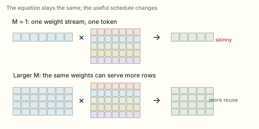
<figure id="fig-geometry" class="wide"><a href="assets/geometry.svg" aria-label="Open full-size diagram: Same calculation, a different number of token rows."><img src="assets/geometry.svg" alt="Same calculation, a different number of token rows. The little tables stand in for much larger matrices. More rows can let a kernel reuse weights, but it also changes which way of dividing up the work makes sense." loading="lazy" width="900" height="450"></a><figcaption><b>Same calculation, a different number of token rows.</b> The little tables stand in for much larger matrices. More rows can let a kernel reuse weights, but it also changes which way of dividing up the work makes sense.</figcaption></figure>

At one token, I read a weight and use it for that one row. With more token rows, I may be able to reuse the same weight for several rows before fetching it again. That reuse can make a different implementation worthwhile.

Imagine getting a book off a shelf. If you're answering one question, you might grab the relevant page and put it away. If you're answering a hundred related questions, keeping the book open makes more sense. The GPU version has more rules, but the reuse idea is similar.

This is why I stopped looking for one kernel that would win everywhere. I needed different approaches for different sizes.

## A quick guide to the numbers I'll be showing

The speedup is **baseline time ÷ my time**. If the baseline takes 10 microseconds and my version takes 8, the ratio is 1.25×. A microsecond is a millionth of a second. Tiny on its own; useful when a model repeats these operations constantly.

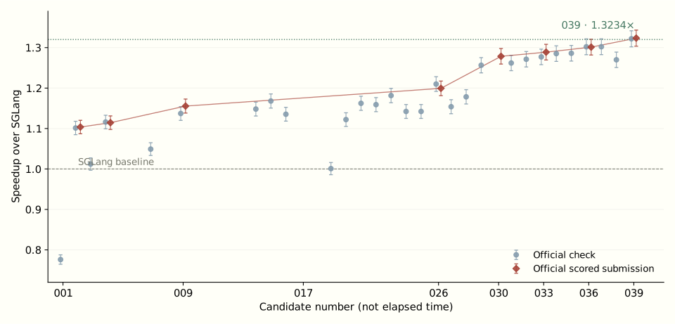
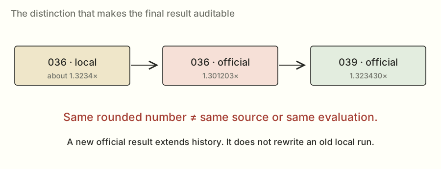
There were also two kinds of official run. A **check** tested correctness and performance without putting the result on the leaderboard. A **scored submission** made a leaderboard attempt. They were separate evaluations and sometimes returned slightly different numbers.

Here's the short version of the route. These are selected milestones; I'll get into what changed below.

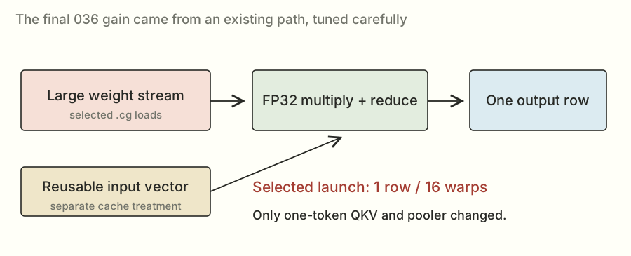
<div class="table-wrap"><table><thead><tr><th>Candidate / change</th><th>Evidence</th><th>Speedup</th></tr></thead><tbody><tr><td><a href="#run-f866e678b7224915">001</a> · First candidate</td><td><span class="tag check">check</span></td><td class="numeric">0.7761×</td></tr><tr><td><a href="#run-cc6781ae999346d3">002</a> · Split router</td><td><span class="tag submit">scored</span></td><td class="numeric">1.1037×</td></tr><tr><td><a href="#run-5a243a8bf9374769">004</a> · Shape-aware router dispatch</td><td><span class="tag submit">scored</span></td><td class="numeric">1.1144×</td></tr><tr><td><a href="#run-1eb88f402c9e49ff">009</a> · Packed high/low router</td><td><span class="tag submit">scored</span></td><td class="numeric">1.1555×</td></tr><tr><td><a href="#run-eb6210fc448642f8">026</a> · Expanded method bundle</td><td><span class="tag submit">scored</span></td><td class="numeric">1.1993×</td></tr><tr><td><a href="#run-f047171bd8e24058">029</a> · Measured best-of plan</td><td><span class="tag check">check</span></td><td class="numeric">1.2564×</td></tr><tr><td><a href="#run-f532c7ddea4149a4">030</a> · Atomic router</td><td><span class="tag submit">scored</span></td><td class="numeric">1.2785×</td></tr><tr><td><a href="#run-54eb1a07e4014863">033</a> · Cluster QKV</td><td><span class="tag submit">scored</span></td><td class="numeric">1.2888×</td></tr><tr><td><a href="#run-d296d0c1b1774e5e">036</a> · Streaming vector + selected layouts</td><td><span class="tag submit">scored</span></td><td class="numeric">1.3012×</td></tr><tr><td><a href="#run-f7219946bf314f37">039</a> · PDL + library choices + skinny QKV</td><td><span class="tag submit">scored</span></td><td class="numeric">1.3234×</td></tr></tbody></table></div>

<figure id="fig-progress" class="wide"><a href="assets/progress.svg" aria-label="Open full-size diagram: How the scores changed as I kept experimenting."><img src="assets/progress.svg" alt="How the scores changed as I kept experimenting. Blue dots are official checks; red diamonds are scored submissions. The little vertical bars show the reported uncertainty. Candidate numbers run left to right, so this is an experiment map rather than a timeline." loading="lazy" width="900" height="450"></a><figcaption><b>How the scores changed as I kept experimenting.</b> Blue dots are official checks; red diamonds are scored submissions. The little vertical bars show the reported uncertainty. Candidate numbers run left to right, so this is an experiment map rather than a timeline.</figcaption></figure>

The line makes this look more orderly than it felt as an engineering problem. There were plenty of branches between those points. Some ran correctly and were slow. Some didn't run at all. I kept both kinds in the <a href="#every-experiment">full experiment log</a>.

One more wrinkle: the final competition number combines the six loads. Inside a load, it adds the five projection times with the specified weights. Then it combines the six speedup ratios using a **geometric mean**: multiply the ratios and take the sixth root.

Why do that? Consider a simpler example with two loads. Make one twice as fast and the other half as fast. Their ratios are 2 and 0.5. Multiplying gives 1, so the geometric mean is 1: no overall win by that measure. An ordinary average would give 1.25 and make that trade look much nicer than it is.

You can play with one load here while leaving the other five unchanged:

<section class="interactive" aria-label="Geometric mean score calculator"><div class="eyebrow">Try the aggregation</div><p>Change one load’s speedup. The other five are held at 1.00×.</p><label for="load-speed">One load: <output id="load-speed-value" for="load-speed">1.30×</output></label><input id="load-speed" type="range" min="0.5" max="2" step="0.01" value="1.3"><p id="score-result" class="result" aria-live="polite"></p><p class="small">Illustrative calculator, not a prediction of a kernel’s performance.</p></section>

My eventual 1.3012× result worked out to about **23.15% less aggregate time**. The later 1.3234× result worked out to about **24.44% less time**. The speedup ratio and the percentage of time saved are different ways of describing the same improvement.

<details class="deep"><summary>The exact scoring formula, if you're curious</summary><p>Within load ℓ, the ratio is the weighted baseline time divided by the weighted candidate time. All five projection families have listed weight 62 in this task, so that common factor cancels. The overall result is the geometric mean of the six load ratios.</p><div class="equation">S<sub>ℓ</sub> = Σᵢ wᵢt<sub>base,i</sub> / Σᵢ wᵢt<sub>candidate,i</sub><br>S = exp((1/6) Σ<sub>ℓ=1…6</sub> log S<sub>ℓ</sub>)</div><p>The 036 result reports 4,830.8 μs for the baseline aggregate and 3,712.563851 μs as the candidate's score-equivalent time. These combine workloads; they aren't the time of one GPU launch.</p></details>

## Having lots of workers doesn't help if I give them nothing to do

The GPU I used was an **H200**. The first thing worth understanding about it is that doing arithmetic and getting the numbers to that arithmetic are separate jobs.

You'll also see the name **Hopper**. That's the architecture family this GPU belongs to. Some of the later techniques use features introduced with that family.

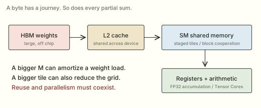
The weights live in a large memory called **HBM**. Closer to the computation are smaller, faster places to keep data: a cache called **L2**, **shared memory** that cooperating threads can use, and **registers** that hold values used by individual threads.

A **thread** is one execution path through the kernel. Threads run in groups of 32 called **warps**. Several warps can belong to a **block**. Blocks are scheduled onto the GPU's processing units, called **streaming multiprocessors**, or SMs.

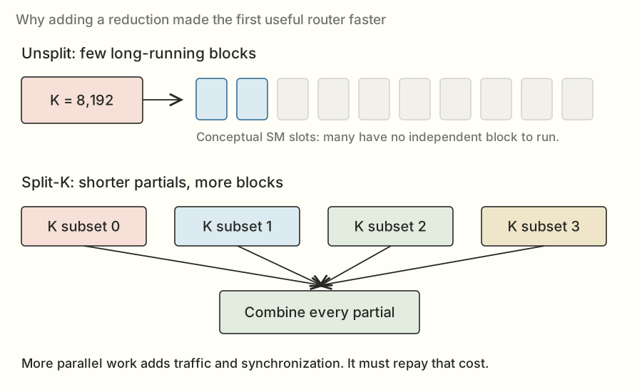
You don't need that whole hierarchy memorized. For the next experiment, the important bit is that **separate blocks give the GPU independent pieces of work to schedule**. A huge amount of work trapped inside a small number of blocks can leave other parts of the GPU with nothing useful to run.

<figure id="fig-memory" class="wide"><a href="assets/memory.svg" aria-label="Open full-size diagram: The numbers have to travel before I can use them."><img src="assets/memory.svg" alt="The numbers have to travel before I can use them. HBM holds the big weight arrays. L2, shared memory, and registers are smaller places closer to the arithmetic. The drawing shows the idea, not the physical size of the hardware." loading="lazy" width="900" height="450"></a><figcaption><b>The numbers have to travel before I can use them.</b> HBM holds the big weight arrays. L2, shared memory, and registers are smaller places closer to the arithmetic. The drawing shows the idea, not the physical size of the hardware.</figcaption></figure>

That's roughly the problem identified in the notes for my first router implementation. The **router** computes scores used to select experts. It had only 256 output features, but each output involved a long sum over K = 8,192 inputs. At small token counts, the chosen output tiles produced too few blocks.

It was a bit like having a large team available and handing out only a couple of enormous tasks. The tasks got done correctly. The rest of the team couldn't do much about how long they took.

That first candidate, `001`, passed correctness and checked at **0.7761×**. The next idea was to break up the long sums.

Before the first win, I want to make the memory and scheduling part as concrete as the algebra. It explains why a mathematically identical program can take such a different amount of time.

## What a matrix looks like in memory

The GPU doesn't see a pretty rectangular table. It sees memory addresses. The table's shape and **strides** tell the program how to turn a row and column into an address.

For a contiguous row-major matrix W with shape `[N, K]`, rows sit one after another. The entry `W[n, k]` is `n × K + k` elements from the beginning. If each element occupies two bytes, the byte offset is `2 × (n × K + k)`.

For the small weight matrix from the earlier example, the stored sequence is:

```text
Logical rows:    [ 4, -1 ]  [ 1, 2 ]  [ -2, 3 ]
Flat storage:      4  -1      1  2      -2  3
Element offset:   0   1      2  3       4  5
```

A **stride** is the distance, in elements, required to move one step along an axis. This W has row stride 2 and column stride 1. Its transpose can be described as shape `[2, 3]` with strides `[1, 2]`, using the same underlying storage. A contiguous copied transpose instead stores `4, 1, -2, -1, 2, 3` in a new array. Same logical transposed matrix; different storage order.

That distinction is why “I transposed it” isn't a complete performance explanation. I need to say whether I changed the view, made a copy, or packed values into a tile-specific arrangement, and which addresses the timed kernel will actually read.

### Coalescing: think about a group of lanes' addresses

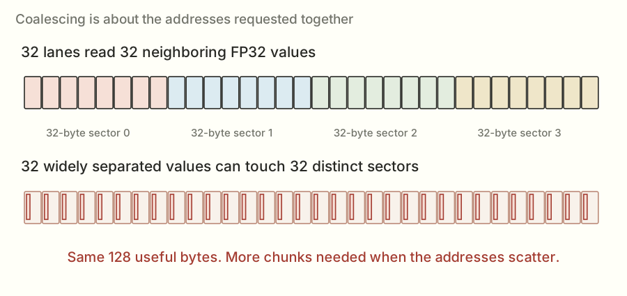
GPU memory is transferred in chunks. If neighboring lanes request neighboring values, the hardware can service them using a compact set of memory sectors. This is **coalescing**. A scattered request can require more sectors to deliver the same useful data.

For an aligned illustrative read of 32 FP32 values, one per lane, the useful payload is 128 bytes. Consecutive addresses cover four 32-byte sectors. If those 32 lanes instead touch widely separated locations in distinct sectors, the request could need 32 sectors for the same 128 useful bytes. Cache reuse and the actual instruction path can change the traffic, but the address calculation explains why the access pattern matters.

<figure id="fig-coalescing" class="wide"><a href="assets/coalescing.svg" aria-label="Open full-size diagram: Neighboring addresses need fewer memory sectors."><img src="assets/coalescing.svg" alt="Neighboring addresses need fewer memory sectors. This is an aligned FP32 teaching example, not a traffic trace from the winning kernel. The boxes in the two rows use different physical scales: the labels give the byte counts." loading="lazy" width="900" height="450"></a><figcaption><b>Neighboring addresses need fewer memory sectors.</b> This is an aligned FP32 teaching example, not a traffic trace from the winning kernel. The boxes in the two rows use different physical scales: the labels give the byte counts.</figcaption></figure>

This is a group property. A lane reading values sequentially over time doesn't guarantee that the whole warp's reads are coalesced at one instruction. I have to inspect what all the active lanes request together.

The original W layout makes consecutive K entries in one row adjacent. A different kernel might want adjacent output features at one K step. Those are separated in the original layout. Packing can put the values that the kernel consumes together next to each other without changing their numerical values.

### Tiling: load a small piece and use it more than once

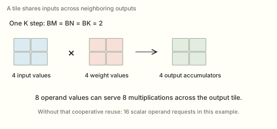
Suppose a block computes a `2 × 2` output tile, and I consider two K terms at a time. It needs a `2 × 2` input tile and a `2 × 2` weight tile: eight distinct operand values. Those values contribute to eight multiplications across four output cells.

If I computed each output cell separately and fetched both operands for both of its K terms without reuse, I'd request sixteen operand values. Cooperative tiling lets neighboring outputs share the values they have in common. This little count illustrates reuse; a real baseline may already benefit from caches and more sophisticated tiling.

<figure id="fig-tiling" class="wide"><a href="assets/tiling.svg" aria-label="Open full-size diagram: Use an operand again before fetching it again."><img src="assets/tiling.svg" alt="Use an operand again before fetching it again. A two-by-two output tile shares input and weight values across neighboring dot products. The little count assumes no other reuse; an actual baseline can already benefit from caches." loading="lazy" width="900" height="450"></a><figcaption><b>Use an operand again before fetching it again.</b> A two-by-two output tile shares input and weight values across neighboring dot products. The little count assumes no other reuse; an actual baseline can already benefit from caches.</figcaption></figure>

For general tile sizes BM, BN, and BK, a K step brings in about `BM×BK + BK×BN` operand elements and performs about `2×BM×BN×BK` useful floating-point operations. With two-byte BF16 operands and ignoring other traffic, the ratio is `BM×BN / (BM + BN)` FLOPs per operand byte for that tile step.

Larger output tiles improve that simplified reuse ratio. But they also need more accumulator state and operand storage. If a block owns too much work, fewer blocks may fit on an SM or the grid may have too few independent blocks. Tiling is a balancing problem, not a proof that the biggest tile wins.

<section class="interactive" aria-label="Explore tile geometry"><div class="eyebrow">Reuse versus the work grid</div><p>Use the real pooler dimensions M=16, N=4,096, K=8,192, and change an illustrative output tile.</p><label for="tile-bm">BM </label><select id="tile-bm"><option value="8">8</option><option value="16" selected>16</option><option value="32">32</option><option value="64">64</option></select> <label for="tile-bn">BN </label><select id="tile-bn"><option value="16">16</option><option value="32" selected>32</option><option value="64">64</option><option value="128">128</option></select><div id="tile-summary" class="result" aria-live="polite">16×32 tiles → 128 output blocks.</div><p id="tile-reuse" class="small">Full-tile operand reuse model: 10.67 FLOPs per BF16 operand byte.</p><p class="small">Geometry calculator only. These are not measured configurations or a runtime prediction. The model ignores scratch, outputs, cache effects, instruction granularity, and scheduling costs.</p></section>

There are several levels of tiling. Blocks own output regions. Warps cooperate on smaller regions. Threads hold parts of the accumulators in registers. Reusing a value from a register can avoid repeatedly loading it from shared memory, just as shared-memory reuse can avoid repeatedly fetching it from a farther-away level.

### Shared memory has a layout problem too

Putting data in shared memory doesn't make every access equally cheap. It is organized into banks. In the usual 32-bit-word view of NVIDIA shared memory, a useful simple model has 32 banks with successive words mapping to successive banks. Requests for different addresses in the same bank can need extra servicing. Multiple lanes reading the same address are a broadcast case, which is different from a conflict among distinct addresses.

For a concrete layout calculation, let lane j read word `32×j`. Its bank index is `(32×j) mod 32 = 0`, so all those distinct words land in one bank. Add padding so the stride is 33 words and the bank index becomes `(33×j) mod 32 = j` for lanes 0 through 31. The logical values can stay the same while the bank mapping changes.

Real matrix-load instructions and wider accesses have additional details. This example explains the purpose of padding and **swizzling**: alter the address layout so the intended cooperative read pattern works better. It isn't a reason to change an arbitrary array's stride and assume performance improved. I still need the exact consuming instructions and a timing.

### Enough active work, with enough resources

An SM has finite registers, shared memory, and thread capacity. A block that needs more of one resource can reduce the number of blocks resident at once. **Occupancy** measures active warps relative to the hardware's maximum, but occupancy is only part of the picture.

More active warps can help hide a wait by giving the scheduler other work to issue. A kernel with enough instruction-level work may also make good progress at lower occupancy. Meanwhile, high occupancy doesn't compensate for a scattered memory pattern or too much redundant traffic.

That is why the statement “the GPU was underused” needs a mechanism. Was the grid too small? Were resources limiting residency? Were warps waiting on data? Was arithmetic padded away on invalid token rows? Timings can show a candidate lost; counters and controlled experiments help identify which explanation is right. I didn't have those counters on the Runpod host, so I kept the difference between a measured outcome and a plausible cause.

The <a href="https://docs.nvidia.com/cuda/cuda-c-best-practices-guide/index.html">CUDA Best Practices Guide</a> is the reference for coalescing and shared-memory access rules. The numerical layouts above are my small worked examples.

## A rough way to ask how much room was left

Before spending another round on a kernel, I wanted a rough sense of what could be limiting it. The **roofline** idea compares useful arithmetic with data movement.

There are about `2MNK` floating-point operations in a matrix multiplication by the usual counting convention: multiply and add count separately. For an individual dot product starting without a zero accumulation, the exact scalar count can be K multiplies and K−1 adds. The conventional `2MNK` count is useful for throughput comparisons; it isn't a count of GPU instructions. One matrix instruction can do many of those operations at once.

If a computation needs F FLOPs and the applicable compute throughput is P FLOPs per second, `F/P` is an optimistic compute time. If it must move B bytes through a memory level with bandwidth Q bytes per second, `B/Q` is an optimistic movement time. If movement and compute overlap, a simple lower-bound model is their maximum, not automatically their sum. Dependencies and overhead can make the real time larger.

For the pooler with M = 16, N = 4,096, and K = 8,192, the BF16 weight payload is:

<div class="equation">2 × 4,096 × 8,192 = 67,108,864 bytes<br>2 × 16 × 4,096 × 8,192 = 1,073,741,824 FLOPs</div>

That's 64 MiB of weights, or about 67.1 decimal MB. A **MiB** is 1,048,576 bytes; a decimal **MB** is 1,000,000. I keep that distinction explicit when dividing bytes by a bandwidth quoted in decimal units.

Using the simplified assumptions in my saved derivation—4.8 trillion bytes per second and 989 trillion applicable operations per second—the weight-only movement bound is about **13.98 μs**, while the arithmetic bound is about **1.09 μs**. Those are optimistic model inputs, not a measurement that my kernel reached either peak.

The task's own floor calculation includes input and output traffic as well as weights. This deliberately simpler weight-only calculation isolates why the large fixed weight stream matters, so its number can differ slightly from the full task floor.

Now change only M to 256. The original weight matrix has exactly the same byte size, but useful arithmetic grows sixteenfold. The simplified compute bound becomes about **17.37 μs**. The balance changes even though the layer name stays “pooler.”

Divide `2MNK` by the weight payload `2NK`, and the result is **M FLOPs per weight byte**. That's the weight-only arithmetic intensity. It ignores activations, outputs, scratch, metadata, rereads, and access inefficiency. It is useful for understanding why token count changes the regime, not for claiming I measured the actual HBM traffic.

The handoff also had empirical read probes: about **3.84 μs for 8.4 MB**, **5.79 μs for 16.8 MB**, **10.43 μs for 37.7 MB**, and **16.65 μs for 67 MB**. These were observed timings in that lab, not universal hardware limits. They gave me a practical comparison point alongside the ideal arithmetic.

If a weight-streaming path is already near a useful measured floor, doubling its arithmetic throughput might save very little. If it is far above that comparison point, there may be scheduling, traffic, or overhead worth investigating. Neither observation tells me a particular new kernel will win. It helps me choose a question worth testing.


## My first useful win: split up the sum

Suppose I need to add up a long list of products. Instead of giving one group the whole list, I can give several groups different pieces. Each computes a partial sum. Then I add the partial sums together.

That's **split-K**. The K dimension is the long input dimension, and I'm splitting the work along it.

<figure id="fig-splitk" class="wide"><a href="assets/splitk.svg" aria-label="Open full-size diagram: Break a long sum into pieces, then add the pieces."><img src="assets/splitk.svg" alt="Break a long sum into pieces, then add the pieces. The empty slots illustrate why too few independent blocks can leave the GPU underused. They are a sketch, not a recorded occupancy trace. Combining the partial answers still costs time." loading="lazy" width="900" height="450"></a><figcaption><b>Break a long sum into pieces, then add the pieces.</b> The empty slots illustrate why too few independent blocks can leave the GPU underused. They are a sketch, not a recorded occupancy trace. Combining the partial answers still costs time.</figcaption></figure>

### A reduction, worked out with small numbers

A **reduction** combines a collection of values into fewer values, often by adding them. The dot product's final sum is a reduction. The output can be one scalar even when thousands of input terms contribute.

Use this small dot product:

<div class="equation">x = [1, 2, 3, 4]<br>w = [5, 6, 7, 8]<br>x · w = 5 + 12 + 21 + 32 = 70</div>

One split could compute the first two terms, getting 17. A second could compute the other two, getting 53. Add their partials and the answer is still 70 in exact arithmetic. The real router used an interleaved K-tile assignment; this contiguous two-piece example is just the simplest way to see the mathematical identity.

The important requirement is that every intended K term is included exactly once. Overlapping splits would double-count work; missing a split would drop terms. Masks also have to exclude padded entries without excluding valid ones.

### How splitting changes the grid

For a tile-based output kernel, a simplified block count is `ceil(M/BM) × ceil(N/BN)`. **ceil** means round up: seventeen rows with a sixteen-row tile need two tiles, not one. A split axis with S pieces can multiply that grid by S.

Consider an illustrative router with M = 16, N = 256, BM = 16, and BN = 64. The unsplit output grid has `1 × 4 = 4` blocks. Thirty-two splits would expose 128 blocks. That is a large scheduling change even though the mathematical output still has only `16 × 256 = 4,096` numbers.

These are example settings to explain the count, not a claim that every candidate used them. The selected plan in each source names the actual split and tile settings for that range.

More blocks do not create more useful mathematical work. They redistribute the same reduction and add some overhead. The win depends on how much idle capacity this redistribution makes useful, how much work remains per block, and how expensive the final combination is.

### The temporary array is a real cost

With S = 32 splits, M = 16 token rows, N = 256 outputs, and four-byte FP32 partials, the temporary has:

<div class="equation">32 × 16 × 256 × 4 = 524,288 bytes<small>512 KiB of partial answers for a final output of only 16 KiB</small></div>

Writing those partials once and reading them once is about one MiB of payload traffic, before other accesses or transaction inefficiency. The combine kernel has its own launch and execution costs. Cache behavior can affect where traffic is served, so payload counting is not a bus-counter measurement.

At a large M, there may already be many output tiles. Splitting can still add scratch and synchronization without solving a shortage of blocks. That explains why “split more” was a hypothesis for a regime, not the direction of unlimited improvement.

### Why a last-block scheme was more complicated than it sounded

One later idea let blocks write partials and update a completion counter. The last block to arrive would read the others' partials and finish the output, avoiding a separate final launch.

But a counter is not enough by itself. The final reader needs the partial writes to be visible before it reads them. The protocol has to use the right ordering and synchronization, and every replay needs a fresh counter. Otherwise the code can work once and fail later or read unfinished data.

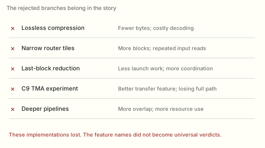
Even a correct protocol still writes partials, updates counters, waits for readiness, and reads the partials back. Avoiding a launch is useful only if those costs are better than the path it replaces. The tested last-block variants did not beat the atomic incumbent.

<details class="deep"><summary>Pause: if I double the split count, does the runtime halve?</summary><p>No. The per-split arithmetic may shrink, but launch, scheduling, scratch traffic, and combination costs don't shrink the same way. Too many tiny pieces can leave more coordination than useful work. The best split count depends on the shape and the full implementation.</p></details>


In candidate `002`, small-token router ranges used sixteen splits. Each block worked on its assigned K tiles and wrote its partial answer into a temporary GPU array. A second kernel added the partials to produce the final output.

Notice the trade: I added a temporary array, extra memory traffic, and another launch. Launching a kernel means asking the GPU to start that program, which has a cost of its own. The hope was that having more useful blocks running would save more time than the extra steps cost.

It did. The official check returned **1.1014×**, and the scored submission returned **1.1037×**.

That was the first useful lesson: a program with more steps can finish sooner if those steps let the hardware work more effectively.

<details class="deep"><summary>Show me the actual split-router code</summary>

<figure class="code-figure"><figcaption>002: partition the router’s K tiles · <a href="evidence/experiments/002-split-router.py">exact source</a> · lines 50–70</figcaption><pre><code class="language-python" data-exact-source="true">def _router(X, HI, LO, Y, M: tl.constexpr, N: tl.constexpr, K: tl.constexpr,
            BM: tl.constexpr, BN: tl.constexpr, BK: tl.constexpr, SPLIT: tl.constexpr):
    rows = tl.program_id(0) * BM + tl.arange(0, BM)
    cols = tl.program_id(1) * BN + tl.arange(0, BN)
    kk = tl.arange(0, BK)
    hi_acc = tl.full((BM, BN), 0, tl.float32)
    lo_acc = tl.full((BM, BN), 0, tl.float32)
    for start in range(tl.cdiv(K, BK * SPLIT)):
        k = (start * SPLIT + tl.program_id(2)) * BK + kk
        x = tl.load(X + rows[:, None] * K + k[None, :],
                    (rows[:, None] &lt; M) &amp; (k[None, :] &lt; K), other=0)
        offsets = k[:, None] * N + cols[None, :]
        mask = (k[:, None] &lt; K) &amp; (cols[None, :] &lt; N)
        hi = tl.load(HI + offsets, mask, other=0)
        lo = tl.load(LO + offsets, mask, other=0)
        hi_acc += tl.dot(x, hi)
        lo_acc += tl.dot(x, lo)
    tl.store(Y + tl.program_id(2) * M * N + rows[:, None] * N + cols[None, :], hi_acc + lo_acc,
             (rows[:, None] &lt; M) &amp; (cols[None, :] &lt; N))

</code></pre></figure>

</details>

But the win wasn't uniform. The smaller-token router cases benefited, while the 256-token case regressed. At larger token counts, there was already more independent output work. Splitting K still charged me for combining partial answers, even when I needed its parallelism less.

So the next question became: where should I use this, and where should I leave the existing path alone?

### Reading the split-router kernel with the equation beside it

The short source excerpt can look dense if Triton is new, so I'll connect it back to `Y[m,n] = Σₖ X[m,k]W[n,k]`.

`tl.program_id(0)` identifies which token tile this program owns. Multiplying it by BM and adding `tl.arange(0, BM)` makes a vector of token-row indices. The second program ID does the same job for BN output columns. The third program ID identifies the K split.

`tl.arange` describes a logical array of indices for the compiler. It does not launch that many independent CPU threads. Triton maps these logical elements and their operations onto the GPU program's warps and lanes.

Now look at the K-index expression: `(start * SPLIT + program_id(2)) * BK + kk`. For the 002 small-token router settings, BK is 64 and SPLIT is 16. Split zero handles K positions 0–63 on its first loop step, then 1,024–1,087 on its next. Split one begins with 64–127, then 1,088–1,151. Across all sixteen splits and eight loop iterations, the 8,192 K positions are covered.

Each loop loads an input tile of shape `[BM, BK]` and two weight tiles of shape `[BK, BN]`, one for the high contribution and one for the low. Two dot products update FP32 accumulators of shape `[BM, BN]`. After the local K work, the program stores its combined partial in the slice owned by its split.

The **mask** arguments say which logical entries are valid. A token tile of sixteen rows may be used for a smaller actual M. Those extra rows must not load or store outside the intended array. Masked values can be supplied as zero for the arithmetic, but the implementation must still write all valid outputs.

The following sum kernel walks the split axis, adding every partial for each valid output cell. Its mathematical role is exactly the little `17 + 53 = 70` example. Most of the complexity is now about assigning addresses and work, rather than changing the operation.

### Why an empty scratch buffer could be okay here

The split path allocated its partial tensor without filling it with zeros. That's valid only because each required partial location is freshly written by its owner before the sum kernel reads it. The previous contents don't contribute.

The atomic path is different: a block reads-modifies-writes a shared destination by adding to what is already there. Its starting contents are part of the answer, so they must be initialized correctly. “This allocation can be empty” is a property of how the kernel uses it, not a general performance rule.

### Preparation is not secretly computing the answer

The task separated `prepare(weights)` from the timed entry point. Preparation could transpose or pack fixed weights, compile extensions, and reserve reusable state. It did not receive the evaluated activations needed to compute their outputs.

For example, packing W into output-feature tiles preserves information I will need for any future X. Precomputing Y for an input I haven't received is impossible without changing the problem. Reusing Y from a previous X would be wrong. That is the clean boundary behind the layout experiments.

The saved contract gave preparation a finite budget, including up to 300 seconds for that phase. Native compilation also had to fit the overall evaluation lifecycle. A fast method that needed an unbounded search or manual setup outside the allowed environment would not be a usable submission.

Inside the timed call, dispatch could use known shape and configuration. Pulling activation values back to the CPU to decide what to do would introduce host synchronization and conflict with the captured execution requirements. The selected routes used the geometry of the job, not a lookup of evaluated answers.


## I started picking a method based on the job

The word for this is **dispatch**. It just means “look at the input, then choose which implementation to run.”

At one token, a direct **matrix-vector** calculation can make sense. That's matrix multiplication with only one input row; you'll see it called GEMV in the code. With more rows, a tiled matrix-multiplication kernel can reuse data. At other sizes, the existing library can be the best choice.

Candidate `003` tried a more selective vector arrangement and checked at **1.0121×**. Candidate `004` adjusted the router ranges and selected vector paths more carefully. It scored **1.1144×**.

These were whole candidate programs, so I can't subtract one score from another and claim that every bit of the difference came from a single change. What the results did show was that choosing useful regions for different methods was worth pursuing.

This also explains why I'll keep saying “at this size.” A method can be a good answer for sixteen tokens and a poor answer for two hundred and fifty-six. Calling it a good or bad kernel without the size leaves out half the story.

## A small detour: the numbers themselves have formats

Before the next router change, there's one more idea we need: how the GPU stores a number.

**FP32** is a 32-bit floating-point format. **BF16**, or bfloat16, uses 16 bits. Fewer bits mean less storage and different precision. BF16 also works with fast matrix hardware on the GPU, called **Tensor Cores**.

That doesn't mean I can quietly change every FP32 number to BF16 and declare the program faster. The task still has a numerical contract: rules for how close my answers must be to the reference calculation. The router is especially sensitive because its scores help choose experts.

### What a floating-point number is approximating

The computer has a finite bit pattern for each stored value. A **bit** is a binary digit, zero or one; eight bits make a byte. An FP32 value occupies four bytes, while a BF16 value occupies two.

A useful way to understand a normal finite floating-point value is binary scientific notation. In decimal, I might write `1.23 × 10³`. In binary, the stored parts describe a sign, a power of two, and significant binary digits. The **exponent** largely determines the scale; the **significand** determines the detail within that scale.

FP32 has one sign bit, eight exponent bits, and 23 explicitly stored fraction bits. BF16 has one sign bit, eight exponent bits, and seven stored fraction bits. For normal values there's also an implicit leading one. The same exponent width gives BF16 a broad range, but the shorter fraction means much wider spacing between nearby representable values.

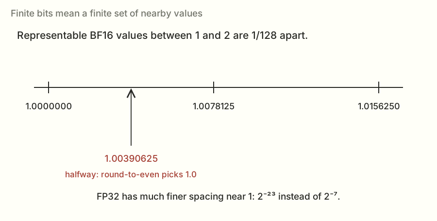
For example, in the interval from 1 up to 2, neighboring BF16 values are separated by `2⁻⁷ = 1/128 = 0.0078125`. Some consecutive choices are `1.0000000`, `1.0078125`, and `1.0156250`. FP32 spacing in that interval is `2⁻²³`, about `0.0000001192`.

The spacing changes with the exponent. BF16 is not “keep a fixed number of digits after the decimal point.” A fixed absolute difference can be tiny at one scale and unrepresentable at another. Zero, subnormal values, infinities, and NaNs have additional representation rules; the task's difficult-input checks matter partly because ordinary values don't exercise every edge case.

<figure id="fig-precision-grid" class="wide"><a href="assets/precision-grid.svg" aria-label="Open full-size diagram: BF16 has visible gaps between representable values."><img src="assets/precision-grid.svg" alt="BF16 has visible gaps between representable values. The axis shows a small range near one. The halfway example uses round-to-nearest, ties-to-even. The spacing changes with magnitude." loading="lazy" width="900" height="450"></a><figcaption><b>BF16 has visible gaps between representable values.</b> The axis shows a small range near one. The halfway example uses round-to-nearest, ties-to-even. The spacing changes with magnitude.</figcaption></figure>

### Inputs, products, accumulators, and outputs are separate choices

An **accumulator** holds the running total while the kernel combines products. A kernel can read BF16 operands, accumulate in FP32, then round the final output into BF16. Those are three different format decisions.

Reading a BF16 value into FP32 doesn't recover information that was already lost when the original value was rounded into BF16. It does let later arithmetic use the wider format. Likewise, a BF16 output tensor doesn't prove intermediate partial sums were combined in FP32; a library might have multiple allowed reduction schemes.

That is why I checked the library's compute and split-reduction settings as well as the final tensor dtype. For the selected cuBLASLt search I requested FP32 compute and the intended compute-type reduction behavior. The correctness tests still had the final say.

### Algebraic rearrangements can change rounding

In exact arithmetic, addition is associative: `(a+b)+c = a+(b+c)`. Floating-point addition rounds to a finite set of values after an operation, so that equality need not survive.

Take these three values in FP32: `100,000,000`, `1`, and `−100,000,000`. The representable spacing around 100 million is larger than one. Adding one to the large positive number can round back to that large number. Subtracting the large number then leaves zero. Cancel the two large numbers first, then add one, and the answer is one.

Both expressions are exactly one in real arithmetic. The computer's finite arithmetic can produce different results because it rounds at different stages. Splitting a reduction or changing which partial arrives first changes those stages. Fused multiply-add and matrix-instruction details can also affect where rounding occurs, so source-level algebra alone doesn't determine the exact bits.

This is not permission to accept any error. The task defines acceptable error against its reference, including row-level conditions and invalid-value checks. An optimization needs to pass that contract across the required inputs.

### Why the high-plus-low router scheme helped

Now I can say more precisely what the high and low parts were doing:

<div class="equation">H = round<sub>BF16</sub>(W)<br>R = W − FP32(H)<br>L = round<sub>BF16</sub>(R)<br>XWᵀ ≈ XHᵀ + XLᵀ</div>

H captures a coarse version of the original weight. R is the residual left after that approximation. L captures much of that residual on its smaller scale. Since the residual is smaller, BF16 can represent details there that it couldn't preserve beside the original large value.

For a convenient exact binary example, take `W = 1.00390625`, halfway between two BF16 values near one. With round-to-nearest, ties-to-even, H is `1.0`. The residual is `0.00390625`, which itself is representable in BF16. Here `H + L` reconstructs this chosen value exactly.

That example explains the idea, not a universal theorem about every FP32 weight. The residual also gets rounded, and the later products and sums introduce their own numerical behavior. The task explicitly permitted this scheme, and I tested it rather than claiming arbitrary lower precision was equivalent.

Contrast that with lossless packing: if I take a stored BF16 value and move its unchanged bits to another address, there's no new approximation at that preparation step. The new execution order can still affect rounding later, but the representation change itself preserved the weight values.

### What a useful correctness check has to catch

Suppose the input row is zero everywhere except feature j, where it equals a power of two. Each output becomes a scaled entry from weight column j. That is a very direct probe of the weight representation. A bad approximation can't rely on cancellation across thousands of random products to look acceptable.

I also need rows where the true output is small. Relative error divides by a scale, so values near zero require the task's specified handling. Replacing the reference's rule with a convenient average error would change what passing means.

And I need repeated calls with new inputs. Passing the first call says nothing about whether a scratch buffer, output, or counter was reset for the second. I'll return to that lifecycle issue in the atomic router and benchmark sections.

### The actual error rule, including what L2 means

The **L2 norm** of a vector is the square root of the sum of its squared entries. For `[3, 4]`, that is `sqrt(9 + 16) = 5`. It's a way to measure the size of the whole vector without letting positive and negative entries cancel. For this whole-output comparison, the array's entries are treated together in the norm.

Relative L2 error divides the norm of the error by the norm of the reference:

<div class="equation">relative error = ‖output − reference‖₂ / ‖reference‖₂</div>

If the reference is `[3, 4]` and my output is `[3.03, 4.04]`, the error vector is `[0.03, 0.04]`, whose norm is 0.05. Divide by the reference norm 5 and the relative error is 0.01, or 1%. That is a whole-vector measure; it doesn't say every individual entry was exactly one percent off.

The saved dense-projection task allowed whole-output relative L2 error up to **1% for the BF16 projections**, and **0.01% for the router**. The reference performed the matrix product in FP64 and converted to the required output type before the supplied comparison. I used the reference implementation rather than substituting a different interpretation of that rule.

Every row also had to satisfy a bound five times its corresponding tolerance. Its denominator was its own reference norm or, if larger, one tenth of the average row norm, with a small numerical floor. That stops a legitimately near-zero row from making a ratio explode while still constraining each row. Otherwise one bad row could hide inside an acceptable whole-array average.

Sparse probe rows had a separate **0.1% bound**. The generator selected them at roughly one row in eight, with at least one at M≥8. The checks also required the exact output shape and dtype and rejected NaN or infinity. Those are different failure modes: the correct shape doesn't excuse the wrong numbers, and a small average error doesn't excuse a broken row or a nonfinite value.

The <a href="evidence/tasks/muse_bf16_proj/reference.py">saved projection reference</a> and <a href="evidence/tasks/muse_bf16_proj/checks.py">comparison code</a> contain the exact rules. All these thresholds are the contract recorded for this investigation.

<details class="deep"><summary>Pause: does an FP32 accumulator make rounded BF16 inputs exact again?</summary><p>No. It gives the running total more precision, but it can't recover information that was already removed from the input representation. That's why operand formats, accumulation, and output rounding need to be discussed separately.</p></details>


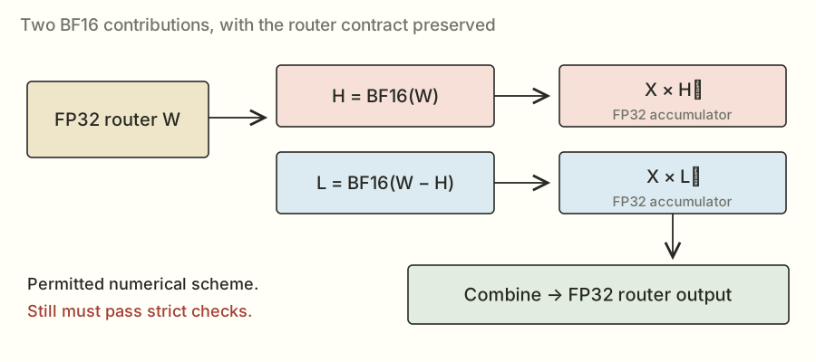
The task allowed a particular high-and-low BF16 scheme for the router weights. First I made a BF16 version of the FP32 weight, called the **high part**. Then I took the leftover difference and made a BF16 version of that, called the **low part**. I multiplied by both parts and combined their contributions in FP32.

<figure id="fig-precision" class="wide"><a href="assets/precision.svg" aria-label="Open full-size diagram: A main contribution and a smaller correction."><img src="assets/precision.svg" alt="A main contribution and a smaller correction. I kept high and low BF16 parts for the task-permitted router scheme and combined the products in FP32. The answer still had to pass the strict reference checks." loading="lazy" width="900" height="450"></a><figcaption><b>A main contribution and a smaller correction.</b> I kept high and low BF16 parts for the task-permitted router scheme and combined the products in FP32. The answer still had to pass the strict reference checks.</figcaption></figure>

Think of writing down a main amount and a smaller correction. Keeping the correction can improve the result compared with keeping only the main amount. It still has to pass the real tests; two BF16 numbers don't magically represent every possible FP32 value exactly.

The other weight changes I'll describe as **lossless packing** are different. Those move existing BF16 values to new addresses without changing their bit patterns. Same numbers, different arrangement.

## Packing the router got me to about 1.15×

Candidate `009` arranged the high and low router weights next to each other in a bigger prepared matrix. That let a library multiplication produce both sets of contributions in one call. A small finishing step added the corresponding high and low outputs.

For smaller token counts I kept the split-router path. For a larger range I used the packed library route. I was building a little collection of methods rather than replacing everything with one kernel.

This candidate checked at **1.1372×** and scored **1.1555×**. The difference between those two numbers was a reminder that check and scored runs are separate measurements. I didn't make another code improvement in between and get to claim the difference as a new technique.

There was still a lot left to do. The bigger dense matrices were reading millions of weights, and their timings made up a substantial part of each load. Making the router faster wasn't going to remove that work.

## I also wandered into attention and experts

This project had a few side quests. They're useful to mention because they explain both what I tried and why the scores can't all be rolled into one big number.

On the attention problem, candidate `005` combined preparation work and scored **1.1323×**. A later split variant checked at about **1.1349×**.

The routed-expert branch started around **0.9945×**, then a version that fused post-normalization work scored **1.1454×**. “Fused” means combining work that would otherwise happen in separate steps. Later tile changes reached **1.2684×** on that problem. A **tile** is a small rectangular piece of a matrix assigned to a group of threads.

When validated components were combined into a whole decode layer, candidate `011` scored about **1.0953×**. The whole-layer number was smaller than some component wins because other work still remained.

There's a useful formula for this, called **Amdahl's law**. If half the original time belongs to a part I make twice as fast, the new total time is one half unchanged plus one quarter for the accelerated part. That's three quarters of the old time, or a 1.33× total speedup. It isn't 2×.

I kept these attention, expert, and layer results in their own tracks. The rest of this article returns to projections. The full side stories are in <a href="notebook.html#chapter-31">notes 31–33</a>.

## Then came a lot of rearranging, measuring, and trying again

One useful direction was **transposing the dense weights ahead of time**. The math is equivalent, but the library sees different layouts and may choose a different way to run the product. Candidate `015` checked at about **1.1680×**.

Other attempts included a Hopper-specific vector route (`014`, about **1.1481× checked**) and wider K tiles (`016`, about **1.1353×**). A bigger tile can reuse more data, but it can also need more memory or leave fewer blocks to run. “Bigger” wasn't a direction I could just keep turning a dial.

The QuACK library attempts brought a more basic problem. Candidates `017` and `018` failed before giving me useful timings. The interface I was using expected a batch dimension: an extra outer dimension around the input matrices. Adding it in `019` and `020` got the calls working. They then checked at about **1.0009×** and **1.1221×**.

The source describes those operands as rank-three arrays. In that API, rank means the number of array axes: batch, rows, and columns. It is different from the linear-algebra meaning of matrix rank, which concerns independent rows or columns.

That distinction matters. A program that didn't run hadn't told me the library was slow. It had told me the integration needed fixing.

I then searched groups of settings more systematically: how many output rows a block owned, how many warps it used, tile sizes, split counts, and library plans. **cuBLASLt**, which shows up a lot in the files, is NVIDIA's matrix-multiplication library interface with more control over layouts and algorithm choices.

<figure id="fig-search" class="wide"><a href="assets/search.svg" aria-label="Open full-size diagram: Try a setting, check it, then see whether the win holds up."><img src="assets/search.svg" alt="Try a setting, check it, then see whether the win holds up. A lucky replay was not enough. Finalists needed more measurements, fresh inputs, nearby sizes, and a complete-candidate test." loading="lazy" width="900" height="450"></a><figcaption><b>Try a setting, check it, then see whether the win holds up.</b> A lucky replay was not enough. Finalists needed more measurements, fresh inputs, nearby sizes, and a complete-candidate test.</figcaption></figure>

Trying lots of settings creates its own trap. If I pick the fastest single timing from a huge search, I might be picking a lucky measurement. So useful finalists needed more runs, new inputs, and nearby sizes. A setting that works at M = 32 also needs sensible behavior around that boundary.

The combined candidate `026` checked at **1.2099×** and scored **1.1993×**. Later, the best-of plan in `029` checked at **1.2564×**. The Claude handoff helped preserve the useful methods, known failures, and remaining opportunities so the next round didn't have to rediscover all of them.

I was making progress. I was also learning that a bundle of good ideas still needs to be tested as a bundle.

## Could I avoid reading all those router partials back?

Remember split-K? I had lots of blocks producing partial sums, then a final kernel reading and adding those sums. Candidate `030` tried a different way to finish: **atomic addition** into the final output.

An atomic add is an update the GPU coordinates so two blocks adding to the same location don't simply overwrite one another. Each split can contribute its answer directly.

<figure id="fig-atomic" class="wide"><a href="assets/atomic.svg" aria-label="Open full-size diagram: Let each split add directly to the answer."><img src="assets/atomic.svg" alt="Let each split add directly to the answer. Candidate 030 removed the separate final reduction pass. It still needed a fresh zero-filled output before those atomic additions." loading="lazy" width="900" height="450"></a><figcaption><b>Let each split add directly to the answer.</b> Candidate 030 removed the separate final reduction pass. It still needed a fresh zero-filled output before those atomic additions.</figcaption></figure>

This removed the dedicated final reduction pass, but it didn't remove every extra step. The output still had to start at zero. If I left yesterday's answer in the buffer and added today's answer to it, the result would be wrong. The zero-fill was part of the call I timed.

<details class="deep"><summary>The code makes that zero-fill explicit</summary>

<figure class="code-figure"><figcaption>Fresh initialization is part of the atomic route · <a href="evidence/winning_source.py">exact source</a> · lines 511–519</figcaption><pre><code class="language-python" data-exact-source="true">def m_ratomic(x, state, layer, n, k, p):
    bm, bn, bk, split = p[:4]
    tuning = {&quot;num_warps&quot;: p[4], &quot;num_stages&quot;: p[5]} if len(p) &gt; 4 else {&quot;num_warps&quot;: 4}
    m = x.shape[0]
    out = torch.zeros((m, n), device=x.device, dtype=torch.float32)
    _paired_router_atomic[(triton.cdiv(m, bm), triton.cdiv(n, bn), split)](
        x, state[&quot;router_interleaved&quot;], out, m, n, k, bm, bn, bk, split, **tuning)
    return out
</code></pre></figure>

</details>

Floating-point sums can also change slightly when contributions arrive in a different order. Atomic addition doesn't solve that numerical issue for me. I still needed the router's correctness checks.

### Follow one output through an atomic router call

Imagine two splits contribute 17 and 53 to an output. If the output starts at zero, atomic additions make it `0 → 17 → 70`, or `0 → 53 → 70` if the other split arrives first. For these small exact integers both orders agree.

If the output instead starts with an old value of 70, the next identical call ends at 140. Each atomic update can be individually coordinated and the complete result can still be wrong. That is why I keep talking about initialization; the atomic operation doesn't decide which computation's answer is currently in the buffer.

A different bug would let two splits each read zero and write their own total without an atomic operation. The final value could be 17 or 53 instead of 70. That's a **race**: the result depends on conflicting accesses without the required coordination.

Now connect that example back to the real paired router. Each block computes FP32 accumulators for high and low output columns, combines the pair belonging to one logical router output, and contributes its split's result. Masks keep it within valid token and output indices. The final output stays FP32.

Atomic updates can arrive in different orders, so the floating-point rounding example from earlier still matters. The implementation needs acceptable numerical behavior across the task's checks, not an assumption that atomic means bitwise deterministic.

### What the code is doing, line by line

In `m_ratomic`, the tuple begins with BM, BN, BK, and the split count. Those control the token tile, output tile, K tile, and number of partial contributors. The wrapper gets the current M from the input shape.

`torch.zeros((m, n), ..., dtype=torch.float32)` creates the initialized output. The launch grid is the number of token tiles, the number of output tiles, and the split count. The kernel receives the prepared interleaved router weights and the fresh input.

The interleaved layout places each output's high and low contributions together. Inside the matrix kernel, the accumulator can be viewed as `[BM, BN, 2]`; summing that last axis combines each pair. The split still owns only part of K, so it atomically adds the resulting `[BM, BN]` tile into the final answer.

The complete captured path includes the initialization and the matrix kernel. A profiler row for only the matrix part would not establish the time of the whole correct call.

### Why I couldn't just use the same trick for every output type

The router's required output is FP32. The dense projections return BF16. Replacing an FP32 partial combine with repeated rounding into a BF16 destination changes the numerical path, and suitable fast atomic mechanisms depend on the data type and hardware.

A technique that wins on this router therefore doesn't automatically transfer to every dense matrix. I need both a valid arithmetic path and a favorable complete cost for the target family. The general idea is to examine combination cost; the specific atomic route earned particular router regions.


Candidate `030` scored **1.2785×**. That became a stronger starting point for the next experiments.

## A tiny matrix and a group of cooperating blocks

There were two more useful pieces before the 1.30× push.

First, the small-token **unpooler** uses a smaller output slice. In that region, FlashInfer's **tiny GEMM** implementation was worth keeping. GEMM is the usual library name for general matrix multiplication. The full candidate `031` checked at **1.2620×**, so it wasn't a new overall milestone above `030`; its useful piece was a selected method for a particular size.

Second, the small-token **QKV projection** still had a lot of weight data to read: roughly 37.7 MB. QKV refers to the query, key, and value representations used around attention. For this section, you can think of it as another projection with an awkwardly small token dimension and a long input dimension.

The custom CUDA path split the K work among cooperating blocks and combined their partial results through **distributed shared memory**. Ordinary shared memory lets threads in a block cooperate. Hopper's **thread-block clusters** let a selected group of blocks cooperate across their shared-memory regions too.

<figure id="fig-cluster" class="wide"><a href="assets/cluster.svg" aria-label="Open full-size diagram: A group of blocks can combine their answers nearby."><img src="assets/cluster.svg" alt="A group of blocks can combine their answers nearby. The earlier QKV path used cp.async, ldmatrix, and mma.sync. The cluster barriers made sure the shared partials were ready, and that their storage stayed alive long enough." loading="lazy" width="900" height="450"></a><figcaption><b>A group of blocks can combine their answers nearby.</b> The earlier QKV path used cp.async, ldmatrix, and mma.sync. The cluster barriers made sure the shared partials were ready, and that their storage stayed alive long enough.</figcaption></figure>

The blocks couldn't just read each other's partials whenever they felt like it. They needed a **barrier**, a point where they waited until the required work was ready. They also needed to keep that shared storage alive until every reader was done.

This path used `cp.async` to stage transfers, `ldmatrix` to load matrix pieces, and `mma.sync` to do matrix arithmetic. Those names are the deeper implementation details. The larger idea is: move tiles in, compute partial answers, then combine them nearby without a separate global reduction launch.

### How a pipeline hides waiting

Imagine one tile load takes L units of time and computing on that tile takes C. A simple sequential loop spends roughly `tiles × (L + C)`. An ideal overlapped pipeline can approach a startup cost plus one stage every `max(L, C)` units. That model explains the potential; it ignores contention and synchronization that a real implementation must pay.

For an illustrative four tiles with L = 3 and C = 5, sequential execution would take 32 units. With ideal overlap, loading the next tile during the current computation could finish in about `3 + 4×5 = 23` units. These are made-up teaching units, not timings from my H200.

<figure id="fig-pipeline-lesson" class="wide"><a href="assets/pipeline-lesson.svg" aria-label="Open full-size diagram: Load the next tile while computing this one."><img src="assets/pipeline-lesson.svg" alt="Load the next tile while computing this one. The numbers are illustrative time units for a dependency example. They are not GPU measurements or a promise that a particular pipeline achieves ideal overlap." loading="lazy" width="900" height="450"></a><figcaption><b>Load the next tile while computing this one.</b> The numbers are illustrative time units for a dependency example. They are not GPU measurements or a promise that a particular pipeline achieves ideal overlap.</figcaption></figure>

Overlapping requires separate storage for tiles in flight. With **double buffering**, I can fill one buffer while consuming another, then swap their roles. A deeper stage ring permits more tiles in flight but consumes more shared memory. If a K split has only a few tiles to compute, a very deep pipeline may have little steady-state work over which to repay its startup and resource costs.

That is why adding stages was an experiment. Shared-memory use can reduce residency, and there may not be enough per-block work to make the overlap useful. The deeper QKV sweeps did not establish a useful win over their selected incumbent in that round.

### A transfer being issued does not mean the data is ready

An asynchronous copy lets the program issue a transfer and do other work before waiting for it. The consumer must still wait for the transfer's required completion before using the data. A producer must also avoid overwriting a stage until the consumer is finished with it.

Those are two distinct directions of coordination: **ready to read** and **safe to reuse**. A ring of buffers without the right barriers is a race with extra storage around it.

In the earlier QKV kernel, `cp.async` organized global-to-shared movement. `ldmatrix` loaded staged fragments into the register organization expected by `mma.sync`, which updated FP32 accumulators. Several threads or lanes collectively own fragments; the instruction's layout determines which values belong where.

Tensor Core throughput is attractive because one matrix instruction represents many multiply-accumulate operations. It also imposes requirements: supported fragment sizes, compatible formats, properly arranged operands, and correct completion before the accumulators are consumed. Simply translating the scalar loop into a matrix instruction name doesn't supply the surrounding schedule.

### Reducing inside a block cluster

The earlier cluster design distributed K work across cooperating blocks. Each block produced a local FP32 partial, put it into its shared-memory region, and joined a cluster barrier. Peer partials could then be read and summed to form the output.

A later barrier protected shared-memory lifetime. If one block exited or reused storage before another finished reading it, a logically correct reduction formula would still become an invalid execution.

This trades global scratch traffic and a separate reduction launch for cluster cooperation, peer accesses, barriers, and cluster residency constraints. The trade helped the selected skinny QKV regime. It did not remove the need to check whether the whole cluster schedule was actually faster.

### Why the later TMA/WGMMA kernel was a new experiment

TMA can move tensor tiles through a dedicated transfer mechanism, and WGMMA performs matrix arithmetic across a warp group. A producer/consumer organization separates roles: one part of the program keeps future operands moving; another performs the arithmetic on ready operands.

The later 039 skinny path combined those roles with tensor-map loads, shared staging barriers, FP32 accumulation, and cluster reduction. Its selected instances used three K splits and eight stages. That complete arrangement differed from both the earlier `cp.async` / `mma.sync` implementation and the earlier losing descriptor-based TMA branch.

I can be more specific from the preserved source. A warp group has four warps, or 128 threads. With the selected MW=1 configuration, the native block has 256 threads: a producer-side group and a consumer group. Thread zero issues the TMA transfers. The consumer group waits for a stage to be full, issues the matrix work, waits for its required completion, and has its warp leaders signal that the stage can be reused. Reserving these roles consumes resources too; the new design still had to earn its timing.

The selected BK is 64, so K=8,192 contains 128 K tiles. The three blocks partition those tiles using integer boundaries: 42 tiles, 43 tiles, and 43 tiles. They need not all do an identical number of tiles, but together they must cover every tile exactly once. This is a concrete difference from a design whose applicability guard requires K to divide evenly by its chosen split width.

The code keeps separate “full” and “empty” stage barriers. Full tells the consumer that the required transfers have completed; empty tells the producer that the previous consumer is done with the slot. Their phase changes let the same ring positions be used across multiple iterations without confusing an old completion with a new tile.

The useful question was not whether TMA “is faster” in isolation. It was whether this layout, role division, pipeline, arithmetic, and combine path beat the prior complete method for those shapes. The official result establishes the later bundle's aggregate outcome; isolating each addition's exact percentage requires the corresponding controlled comparisons.


Candidate `033` independently scored **1.2888×**. It kept the cluster method in its useful small-token QKV region and kept other methods elsewhere.

I was close to 1.30×. Getting the rest still took several more branches.

## How I checked whether an idea was actually faster

I edited on my Mac and used a remote **Runpod H200** for the GPU experiments. Runpod let me rent the machine; the lab copied source there, ran the jobs, and copied results back. The submitted kernel didn't need internet access.

The timing setup mattered as much as the GPU. If I ran the exact same inputs and weights repeatedly, some data could stay in fast cache. That might tell me more about a convenient replay than the competition's intended workload.

So the lab used new inputs, rotated separate copies of the weights, and cleared out L2 before timing. It also alternated the order: sometimes baseline first, sometimes my version first.

<figure id="fig-measurement" class="wide"><a href="assets/measurement.svg" aria-label="Open full-size diagram: Give both versions the same timing conditions."><img src="assets/measurement.svg" alt="Give both versions the same timing conditions. I cleared L2 before both measurements and swapped which version ran first. The boxes explain the sequence; their widths are not measured durations." loading="lazy" width="900" height="450"></a><figcaption><b>Give both versions the same timing conditions.</b> I cleared L2 before both measurements and swapped which version ran first. The boxes explain the sequence; their widths are not measured durations.</figcaption></figure>

The calls ran as **CUDA graphs**. A graph records a sequence of GPU operations so it can be replayed with less CPU involvement. Since the judge measured that mode, it was the mode I needed to compare. Timing an ordinary Python call could include different overhead.

The judge also corrected for a fixed replay cost. Locally that correction was recorded at around 4 μs. With operations this short, a small difference in overhead or measurement conditions can move a percentage noticeably.

Correctness wasn't just “try a random input once.” The checks included difficult inputs, unusual values, nearby shapes, and graph replays with fresh inputs. A particularly useful test put one nonzero value in an input row. That exposes a scaled piece of the weights, making it harder for an incorrect weight conversion to hide inside a big random sum.

One limitation: the Runpod host didn't expose the permissions needed for Nsight Compute's hardware counters. I could measure which version won and use timing profiles, but I couldn't claim to have a full counter-based explanation for every loss.

The lab also had an unglamorous cloud-computing lesson: an idle rented GPU can still bill you. The saved notes include an idle billing episode, a credit-related restart failure, and incomplete searches recovered later. Keeping the results locally and checking what actually finished mattered.

### What I mean by a fair paired measurement

A GPU launch is asynchronous: the CPU can finish asking for work before the GPU has finished doing it. A CPU stopwatch around the launch alone can therefore measure the request rather than the computation. The timing path needs the appropriate GPU event and completion handling; the judge's graph-replay benchmark supplied that controlled path.

Suppose the baseline takes 10 μs and my candidate takes 8 μs in one pair. That pair's ratio is 1.25. Another pair might return slightly different times because clocks, scheduling, or the surrounding state changed. Pairing is an attempt to compare nearby observations under similar conditions, and swapping the order reduces a simple first-versus-second bias.

Summarizing several paired ratios is not always numerically identical to taking two unrelated medians and dividing them. I kept the judge's method as the authority for its score and used the local harness to choose candidates worth checking there.

Clearing L2 and rotating weight states also serve specific purposes. Repeating one already-cached weight copy can answer a different question from reading weights under the benchmark's intended conditions. Neither a cold nor warm experiment is universally the right production model; the point here was to match what this competition tested.

### A tiny overhead error can look like a useful win

For a simple illustration, imagine raw event times of 14 μs and 12 μs. Subtract a fixed 4 μs overhead and the adjusted times are 10 and 8, producing 1.25×. Subtract 4.5 μs instead and the ratio is `9.5/7.5`, about 1.2667×.

The underlying raw observations didn't change. The adjustment did. This isn't an explanation proven for the local-to-official gap; it's a numerical example showing why very short calls need careful calibration and why a local result near the target wasn't a guarantee.

Longer measurements can reduce some timer sensitivity, but changing the execution mode or removing required work would create a different benchmark. I needed the correct captured call, enough repetitions, and the same comparison method.

### Fresh graph replay is a correctness test too

A CUDA graph records work to replay. It doesn't entitle the implementation to keep an old evaluated answer. If I change X between replays, Y must follow the new X.

The tiny matrix example makes this easy to see. The first input row `[2, 3]` produces `[5, 8, 5]`. A later input row `[3, 1]` must produce `[11, 5, -3]`. A graph that keeps returning `[5, 8, 5]` is stale, even if it has an impressively short timing.

The same reasoning catches partial buffers and counters that weren't reset. Eager execution can hide a lifecycle mistake if I only check one call. Replaying with new inputs exercises whether the captured structure still performs the right computation each time.

### Search noise changes how I pick a winner

If I test a thousand configurations, one can look unusually fast by chance. Choosing it from its single best run overstates what I learned. That's why the search was a funnel: cheap screening first, more repetitions for promising candidates, fresh correctness, neighboring shapes, then the complete combination.

Overlapping reported intervals don't prove two programs are identical, and a higher point estimate doesn't prove a tiny difference is repeatable. The right response depends on the size and consistency of the evidence. For a clean dispatch, a clearly useful region is easier to justify than continual changes based on very small noisy differences.

When the official record gives an interval, I show it with the point estimate. When an unfinished search gives only a source file or partial log, I keep it unfinished. Those distinctions are part of the technical explanation, not paperwork after it.


## Sometimes moving the same numbers around was enough

The **pooler** was another projection where small-token timings left room to improve. Pooler and unpooler are the task's names for two of the surrounding transformations; for the optimization here, their input and output sizes are what matter. The C2 experiments packed the weight values so each output tile's region was contiguous: the values it needed were next to each other in memory.

Imagine having all the ingredients for one recipe together instead of walking up and down the same aisle to find each one. The actual GPU access rules are more precise, but that's the motivation behind this layout change.

<figure id="fig-packing" class="wide"><a href="assets/packing.svg" aria-label="Open full-size diagram: Keep one tile’s weights together."><img src="assets/packing.svg" alt="Keep one tile’s weights together. The colors trace groups of output features into a new memory arrangement. The original BF16 values stay exactly the same." loading="lazy" width="900" height="450"></a><figcaption><b>Keep one tile’s weights together.</b> The colors trace groups of output features into a new memory arrangement. The original BF16 values stay exactly the same.</figcaption></figure>

The selected small-token settings used output tiles of 32 features and K tiles of 512, with different token tiles and pipeline depths. A **pipeline** tries to fetch a future tile while computing the current one. More stages can help overlap, but each stage needs storage, so deeper isn't automatically better.

Local retests showed useful pooler gains. The combined candidate `034`, though, checked at **1.2852×**, below the earlier scored point for `033`. A faster component hadn't yet given me a better official overall result.

I also tried presenting equivalent products to cuBLASLt in different orientations. One way computes the normal product. Another uses prepared transposed weights. Another computes a swapped product and views the output with rows and columns exchanged.

<figure id="fig-orientations" class="wide"><a href="assets/orientations.svg" aria-label="Open full-size diagram: The library can run equivalent products in different ways."><img src="assets/orientations.svg" alt="The library can run equivalent products in different ways. I tried different layouts while keeping the same logical output. A layout that worked at one size could still need a fallback next door." loading="lazy" width="900" height="450"></a><figcaption><b>The library can run equivalent products in different ways.</b> I tried different layouts while keeping the same logical output. A layout that worked at one size could still need a fallback next door.</figcaption></figure>

Same logical answer, different library choices. Some were useful at a tested size and poor at a neighboring one. For selected swapped-output routes, token counts not divisible by eight fell back to the retained method because the memory alignment wasn't suitable. **Alignment** means where data starts and how rows line up with the boundaries the chosen operations expect.

### Prove the swapped product before worrying about its speed

The equation is `Y = XWᵀ`, with Y shaped `[M,N]`. Transpose both sides and the equivalent product is `Yᵀ = WXᵀ`, shaped `[N,M]`.

I can verify it from a single entry. The original `Y[m,n]` sums `X[m,k] × W[n,k]` over K. The swapped result at `[n,m]` sums `W[n,k] × X[m,k]`. The scalar products are equal term by term. So a transposed view of the swapped result represents the intended Y.

This identity is not a claim that arbitrary matrices commute. It uses a transpose of the complete result and reverses the transposed operands in a specific way. The shapes and output interpretation change together.

Why might it be faster? A library chooses implementations based on descriptors: dimensions, data types, which axis is contiguous, leading dimensions, workspace, and algorithm settings. Equivalent logical results can therefore be presented as different scheduling problems to the library.

The library might already be doing an excellent job. My search was looking for useful cases where a different presentation or a validated algorithm choice did better, not assuming I could improve a mature library everywhere.

### The alignment fallback came from a real byte condition

For the selected swapped-output route, the allocated array has shape `[N,M]` before returning a transposed view. With BF16 entries, successive allocated rows are separated by `2M` bytes.

The selected tiles wanted the relevant sixteen-byte row alignment. If M is a multiple of eight, `2M` is a multiple of sixteen. At M = 17, it is 34 bytes, so consecutive row starts do not preserve that alignment. The source kept the earlier method when the selected swapped route had this unfavorable token-count condition.

Alignment is one reason a result at an exact scored dimension can fail to generalize next door. Tile padding, algorithm-list changes, and resource thresholds can introduce other boundaries too. I tested neighbors because the implementation should behave as a valid shape-dependent method, not as a list of memorized benchmark answers.

### An algorithm index is a position in a list

The later QKV and pooler selections included indices 172 and 290 in their shape-specific C15 enumerations. Those integers are not permanent names for two universally fast algorithms. Change the shape or the environment and a list position can identify a different choice or cease to be valid.

That is why 039 applied the expanded selections to QKV at M=128 and pooler at M=256, while nearby regions retained earlier routes. Broadening a range without validation would change the experiment and its risks.

Search also has practical costs. There is heuristic enumeration, compatibility checking, workspace, compilation for native variants, and enough measurement to distinguish useful finalists. The broad earlier C15 search reached a time limit before completing its intended space. A partial search log wasn't evidence for a completed improvement. The later source needed its own recovered passing results.

### Weight packing and library descriptors solve related but different problems

The packed pooler path explicitly rearranged the original weights into a layout its own kernel consumed. The library-layout work changed the orientation and descriptors used to ask a library for the product. Both preserved the required values, but they incurred different preparation, memory, and execution costs.

The winning submission could use each in a different region. That is why I evaluated the final dispatch as a complete program. Shared preparation, selected fallbacks, and the workload aggregation can matter even when two isolated method timings look attractive.


Candidate `035` checked at **1.2860×**. Still short. I kept the useful pieces and continued looking for something that complemented them.

## The clever ideas that didn't make it

I tried **lossless compression** for the dense weights. If reading weights was expensive, could I read fewer bytes and reconstruct the exact original values inside the kernel?

It was a reasonable question. But decompressing adds work: metadata, bit operations, extra indexing, and temporary values. Some tested versions ran at less than half the incumbent's speed. The smaller byte count didn't pay for everything I added around it.

I also tried narrower router tiles, different arrangements of high and low contributions, and a design where the last block to finish combined partials. These moved costs around without beating the atomic route in the tested configurations.

Then there was the early **TMA** experiment. TMA stands for **Tensor Memory Accelerator**, a Hopper mechanism for moving tensor data. Having better transfer machinery doesn't guarantee the complete kernel will have the right schedule, enough useful work, or a cheap reduction. This particular family didn't give me a useful local win.

<figure id="fig-rejections" class="wide"><a href="assets/rejections.svg" aria-label="Open full-size diagram: The things that sounded useful and still lost."><img src="assets/rejections.svg" alt="The things that sounded useful and still lost. Each idea changed more than one cost. These are the tradeoffs I had to consider, not a claim that hardware counters proved every explanation." loading="lazy" width="900" height="450"></a><figcaption><b>The things that sounded useful and still lost.</b> Each idea changed more than one cost. These are the tradeoffs I had to consider, not a claim that hardware counters proved every explanation.</figcaption></figure>

Deeper QKV pipelines and more pooler refinements also failed to produce a clear next improvement. Some choices were obviously worse; others were close enough that I didn't want to replace a working setting on the strength of one flattering replay.

I kept these failures in the notes. They mattered later, especially because a different TMA design eventually did help. “I tried this feature once” isn't the same as having tested every way to use it.

## The change that finally took me over 1.30×

After all that, the next useful improvement came from revisiting the one-token vector path.

At one token, there isn't much reuse of a weight across token rows. The kernel reads the input vector, reads the weights, multiplies, and sums. The C10 search revisited how many output rows each block owned, how many warps it used, and how it treated the weight stream in cache.

For the selected QKV and pooler entries, the useful configuration was **one output row per block, sixteen warps, and `.cg` weight loads**. The `.cg` setting controls cache behavior; it lets those weight loads use the global caching path without using L1. The much smaller input vector had different reuse needs, so it received different treatment.

<figure id="fig-vector" class="wide"><a href="assets/vector.svg" aria-label="Open full-size diagram: The one-token path was still worth another look."><img src="assets/vector.svg" alt="The one-token path was still worth another look. Candidate 036 updated the first QKV and pooler entries to the selected vector configuration. Other ranges kept their existing choices." loading="lazy" width="900" height="450"></a><figcaption><b>The one-token path was still worth another look.</b> Candidate 036 updated the first QKV and pooler entries to the selected vector configuration. Other ranges kept their existing choices.</figcaption></figure>

The local paired comparisons repeatedly found useful gains in these one-token cases: roughly six percent for QKV and just under five percent for pooler in a later retest. Those are component improvements in that local comparison, not percentages I could simply add to the overall score.

### Read the one-token kernel from addresses to output

The mathematical job is one dot product per output row. With one output row per program, the grid has N programs. `row = program_id(0) * BN + arange(0, BN)` identifies the owned output row or rows; the selected BN is one.

`col = arange(0, BK)` identifies logical K positions. BK is chosen as the next power of two at least as large as K. That makes the reduction structure convenient, and the masks prevent padded positions from contributing when necessary.

The weight address expression is `W + row[:,None] * K + col[None,:]`. The `None` entries introduce axes so row indices and K indices broadcast into a rectangular index table. “Broadcast” here means apply one index along several logical entries, not physically copy the weight array first.

The input address is `X + col`, because this path has just one token row. The code converts loaded values to FP32, multiplies matching positions, and uses `tl.sum(..., axis=1)` to reduce across K. Finally it stores the valid output row, with the required result dtype supplied by the output allocation.

This is the same mathematical dot product from the start of the article. The new details are addresses, masks, formats, and which program owns each sum.

### What changing the warp count could change

Sixteen warps contain 512 threads. For a K of 8,192, an ideal even division would assign about sixteen logical K values per thread. Eight warps would average thirty-two. This is a useful count to build intuition; the compiler's actual mapping and generated instructions determine the real execution.

Changing the warp count can change values held per thread, register allocation, the reduction tree, synchronization, and which blocks can reside together. A larger launch is not simply the old launch with a guaranteed proportional speed increase.

That is why thirty-two warps was a meaningful follow-up test and its regression was meaningful evidence. The measured fact is that the complete 038 candidate checked worse. Without the unavailable counters, I can't assign every part of that loss to one resource limit.

### The input and weights had different reuse needs

At one token, the large weight rows are streamed for their outputs. The small input vector is reused across many output rows. Treating those streams identically in cache isn't automatically optimal.

The selected `.cg` weight-load setting used the global caching path without L1 caching for those loads. The code kept separate eviction treatment for the input vector. A cache policy is a hardware/compiler instruction choice with constraints; unsupported attribute combinations can fail before there is a valid performance result.

The chosen policy and sixteen-warp launch repeatedly helped the selected one-token QKV and pooler cases locally. The final complete candidate was then checked and scored officially. That last step matters: a tidy explanation of why a cache choice might help does not substitute for the result showing that the bundled source actually did.


<details class="deep"><summary>The short kernel behind that change</summary>

<figure class="code-figure"><figcaption>036: the selected one-token streaming kernel · <a href="evidence/winning_source.py">exact source</a> · lines 1354–1370</figcaption><pre><code class="language-python" data-exact-source="true">@triton.jit
def _c10_vector(X, W, Y, N: tl.constexpr, K: tl.constexpr,
                 BN: tl.constexpr, BK: tl.constexpr, CACHE: tl.constexpr):
    row = tl.program_id(0) * BN + tl.arange(0, BN)
    col = tl.arange(0, BK)
    if CACHE == &#x27;&#x27;:
        w = tl.load(W + row[:, None] * K + col[None, :],
                    (row[:, None] &lt; N) &amp; (col[None, :] &lt; K), other=0,
                    eviction_policy=&#x27;evict_first&#x27;).to(tl.float32)
    else:
        w = tl.load(W + row[:, None] * K + col[None, :],
                    (row[:, None] &lt; N) &amp; (col[None, :] &lt; K), other=0,
                    cache_modifier=CACHE).to(tl.float32)
    x = tl.load(X + col, col &lt; K, other=0, eviction_policy=&#x27;evict_last&#x27;).to(tl.float32)
    value = tl.sum(w * x[None, :], axis=1)
    tl.store(Y + row, value, row &lt; N)
</code></pre></figure>

</details>

Candidate `036` combined those two updated entries with the useful packing, cluster, router, tiny-matrix, and library routes from the earlier work.

The official check passed at **1.3020×**. The scored submission passed at **1.3012×**.

That was the 1.30× milestone I had been asking for.

The final program wasn't one heroic replacement for matrix multiplication. It was a set of fairly specific choices about which method should run where.

## What actually ran in the winning version?

At one token, QKV and pooler used the new vector path. Small-token QKV used the earlier cooperating-block kernel. Small-token pooler used its packed weights. Other ranges used the selected library orientations or existing library calls. The router used a direct FP32 path at one token and high/low contributions with atomic accumulation above it.

You can inspect those choices here. Change the token count and watch the selected method change:

<section class="interactive" aria-label="Inspect candidate 036 dispatch"><div class="eyebrow">Read the selected policy</div><label for="route-layer">Projection </label><select id="route-layer"><option value="qkv_gate">qkv_gate</option><option value="o">o</option><option value="pooler">pooler</option><option value="unpooler">unpooler</option><option value="router">router</option></select> <label for="route-m">M </label><input id="route-m" type="number" min="1" max="4096" value="16"><p id="route-result" class="result" aria-live="polite"></p><p class="small">036’s first matching plan entry. Swapped-output library routes can fall back for M not divisible by eight; applicability guards and full fallback code remain in the linked source.</p></section>

<details class="deep"><summary>The exact dispatch entries</summary>

<figure class="code-figure"><figcaption>The dense dispatch regions, before the two C10 entry replacements · <a href="evidence/winning_source.py">exact source</a> · lines 1349–1351</figcaption><pre><code class="language-python" data-exact-source="true">PLAN[&#x27;qkv_gate&#x27;] = [(1, &#x27;vector&#x27;, (1,4)), (16, &#x27;cluster&#x27;, (8,3,2,128)), (32, &#x27;c7lt&#x27;, (3,8)), (1&lt;&lt;30, &#x27;cublas&#x27;, ())]
PLAN[&#x27;pooler&#x27;] = [(1, &#x27;vector&#x27;, (1,8)), (16, &#x27;c2packed&#x27;, (16,32,512,2,4)), (32, &#x27;c2packed&#x27;, (32,32,512,2,3)), (64, &#x27;trans&#x27;, ()), (128, &#x27;c7lt&#x27;, (3,1)), (1&lt;&lt;30, &#x27;c7lt&#x27;, (0,3))]
PLAN[&#x27;unpooler&#x27;] = [(1, &#x27;vector&#x27;, (1,8)), (8, &#x27;flashinfer&#x27;, (&#x27;tinygemm&#x27;,)), (128, &#x27;trans&#x27;, ()), (1&lt;&lt;30, &#x27;c7lt&#x27;, (3,0))]</code></pre></figure><p class="small">The final two lines replace QKV and pooler’s first entries with <code>(1, 'c10vector', (1, 16, '.cg'))</code>. Full applicability and fallback logic stays in the exact source.</p>

</details>

If you want to see where the time went, here's a more useful picture than the final score alone. These are the saved **official 036 timings**. Each group shows baseline and candidate times for one load. Lower is better.

<section class="interactive" aria-label="Explore official shape timings"><div class="eyebrow">Where the time went</div><label for="load-select">Choose a group of inputs </label><select id="load-select"><option value="0">decode 1 · M = 1</option><option value="1">decode 16 · M = 16</option><option value="2">decode 32 · M = 32</option><option value="3">verify 1 · M = 8</option><option value="4">verify 16 · M = 128</option><option value="5">verify 32 · M = 256</option></select><p class="small">Official 036 timings · baseline versus my version · microseconds (μs) · lower is better</p><div id="shape-bars" aria-live="polite"></div><p id="load-ratio" class="result"></p></section>

Some shapes improved a lot. A few were slightly worse. The full score came from all of them together.

<details class="deep"><summary>Inspect all thirty official shape timings</summary><div class="table-wrap"><table class="shape-table"><caption>All thirty scored shapes · candidate 036 · official timings</caption><thead><tr><th>Load</th><th>Layer</th><th>M / N / K</th><th>Baseline μs</th><th>036 μs</th><th>Ratio</th></tr></thead><tbody><tr><td>decode 1</td><td>qkv_gate</td><td class="numeric">1 / 2,304 / 8,192</td><td class="numeric">14.080</td><td class="numeric">10.077</td><td class="numeric gain">1.397×</td></tr><tr><td>decode 1</td><td>o</td><td class="numeric">1 / 8,192 / 1,024</td><td class="numeric">6.784</td><td class="numeric">5.490</td><td class="numeric gain">1.236×</td></tr><tr><td>decode 1</td><td>pooler</td><td class="numeric">1 / 4,096 / 8,192</td><td class="numeric">21.456</td><td class="numeric">16.532</td><td class="numeric gain">1.298×</td></tr><tr><td>decode 1</td><td>unpooler</td><td class="numeric">1 / 1,024 / 4,096</td><td class="numeric">6.912</td><td class="numeric">3.666</td><td class="numeric gain">1.886×</td></tr><tr><td>decode 1</td><td>router</td><td class="numeric">1 / 256 / 8,192</td><td class="numeric">10.528</td><td class="numeric">3.770</td><td class="numeric gain">2.792×</td></tr><tr><td>decode 16</td><td>qkv_gate</td><td class="numeric">16 / 2,304 / 8,192</td><td class="numeric">14.128</td><td class="numeric">12.971</td><td class="numeric gain">1.089×</td></tr><tr><td>decode 16</td><td>o</td><td class="numeric">16 / 8,192 / 1,024</td><td class="numeric">6.656</td><td class="numeric">6.700</td><td class="numeric loss">0.993×</td></tr><tr><td>decode 16</td><td>pooler</td><td class="numeric">16 / 4,096 / 8,192</td><td class="numeric">21.104</td><td class="numeric">18.073</td><td class="numeric gain">1.168×</td></tr><tr><td>decode 16</td><td>unpooler</td><td class="numeric">16 / 8,192 / 4,096</td><td class="numeric">18.624</td><td class="numeric">18.126</td><td class="numeric gain">1.027×</td></tr><tr><td>decode 16</td><td>router</td><td class="numeric">16 / 256 / 8,192</td><td class="numeric">14.720</td><td class="numeric">5.102</td><td class="numeric gain">2.885×</td></tr><tr><td>decode 32</td><td>qkv_gate</td><td class="numeric">32 / 2,304 / 8,192</td><td class="numeric">14.144</td><td class="numeric">13.028</td><td class="numeric gain">1.086×</td></tr><tr><td>decode 32</td><td>o</td><td class="numeric">32 / 8,192 / 1,024</td><td class="numeric">6.784</td><td class="numeric">6.665</td><td class="numeric gain">1.018×</td></tr><tr><td>decode 32</td><td>pooler</td><td class="numeric">32 / 4,096 / 8,192</td><td class="numeric">21.952</td><td class="numeric">18.839</td><td class="numeric gain">1.165×</td></tr><tr><td>decode 32</td><td>unpooler</td><td class="numeric">32 / 8,192 / 4,096</td><td class="numeric">18.560</td><td class="numeric">17.887</td><td class="numeric gain">1.038×</td></tr><tr><td>decode 32</td><td>router</td><td class="numeric">32 / 256 / 8,192</td><td class="numeric">15.280</td><td class="numeric">5.726</td><td class="numeric gain">2.669×</td></tr><tr><td>verify 1</td><td>qkv_gate</td><td class="numeric">8 / 2,304 / 8,192</td><td class="numeric">13.984</td><td class="numeric">12.594</td><td class="numeric gain">1.110×</td></tr><tr><td>verify 1</td><td>o</td><td class="numeric">8 / 8,192 / 1,024</td><td class="numeric">6.464</td><td class="numeric">6.544</td><td class="numeric loss">0.988×</td></tr><tr><td>verify 1</td><td>pooler</td><td class="numeric">8 / 4,096 / 8,192</td><td class="numeric">21.248</td><td class="numeric">18.066</td><td class="numeric gain">1.176×</td></tr><tr><td>verify 1</td><td>unpooler</td><td class="numeric">8 / 1,024 / 4,096</td><td class="numeric">6.848</td><td class="numeric">4.766</td><td class="numeric gain">1.437×</td></tr><tr><td>verify 1</td><td>router</td><td class="numeric">8 / 256 / 8,192</td><td class="numeric">25.984</td><td class="numeric">5.035</td><td class="numeric gain">5.160×</td></tr><tr><td>verify 16</td><td>qkv_gate</td><td class="numeric">128 / 2,304 / 8,192</td><td class="numeric">17.232</td><td class="numeric">17.089</td><td class="numeric gain">1.008×</td></tr><tr><td>verify 16</td><td>o</td><td class="numeric">128 / 8,192 / 1,024</td><td class="numeric">7.424</td><td class="numeric">7.651</td><td class="numeric loss">0.970×</td></tr><tr><td>verify 16</td><td>pooler</td><td class="numeric">128 / 4,096 / 8,192</td><td class="numeric">24.928</td><td class="numeric">21.066</td><td class="numeric gain">1.183×</td></tr><tr><td>verify 16</td><td>unpooler</td><td class="numeric">128 / 8,192 / 4,096</td><td class="numeric">19.584</td><td class="numeric">18.928</td><td class="numeric gain">1.035×</td></tr><tr><td>verify 16</td><td>router</td><td class="numeric">128 / 256 / 8,192</td><td class="numeric">16.160</td><td class="numeric">6.829</td><td class="numeric gain">2.367×</td></tr><tr><td>verify 32</td><td>qkv_gate</td><td class="numeric">256 / 2,304 / 8,192</td><td class="numeric">20.000</td><td class="numeric">19.936</td><td class="numeric gain">1.003×</td></tr><tr><td>verify 32</td><td>o</td><td class="numeric">256 / 8,192 / 1,024</td><td class="numeric">9.152</td><td class="numeric">9.488</td><td class="numeric loss">0.965×</td></tr><tr><td>verify 32</td><td>pooler</td><td class="numeric">256 / 4,096 / 8,192</td><td class="numeric">30.896</td><td class="numeric">28.949</td><td class="numeric gain">1.067×</td></tr><tr><td>verify 32</td><td>unpooler</td><td class="numeric">256 / 8,192 / 4,096</td><td class="numeric">23.984</td><td class="numeric">23.861</td><td class="numeric gain">1.005×</td></tr><tr><td>verify 32</td><td>router</td><td class="numeric">256 / 256 / 8,192</td><td class="numeric">17.568</td><td class="numeric">8.884</td><td class="numeric gain">1.977×</td></tr></tbody></table></div><p class="small"><a href="evidence/projection_shapes.csv" download>Download the shape data as CSV</a>. Ratios shown here divide displayed shape estimates; the official aggregate retains the evaluator’s paired-ratio method.</p></details>

I saved the exact source and official results rather than just keeping a file named “best.” That's how I could come back later and know which program had actually earned the number. They're linked in the <a href="evidence.html">code and results page</a>.

## The annoying bit: my local run said 1.3234×

The complete 036 bundle looked encouraging in the lab. It measured about **1.0241× against the saved 033 version**, and about **1.3234× against the local SGLang baseline**.

By then my target had moved to 1.32×. So the local number looked like I might already be there.

The official result was **1.3012×**.

<figure id="fig-local-official" class="wide"><a href="assets/local-official.svg" aria-label="Open full-size diagram: The same rounded number, from different runs."><img src="assets/local-official.svg" alt="The same rounded number, from different runs. 036 measured about 1.3234× locally but scored 1.3012× officially. Later, different code in 039 officially scored 1.3234×." loading="lazy" width="900" height="450"></a><figcaption><b>The same rounded number, from different runs.</b> 036 measured about 1.3234× locally but scored 1.3012× officially. Later, different code in 039 officially scored 1.3234×.</figcaption></figure>

The local setup matched important parts of the judge, but it wasn't identical. Machine and driver details, exact baseline behavior, overhead estimates, and ordinary variation could all contribute. I didn't have an experiment that proved one cause explained the whole gap.

So I kept the local number labeled local and used the official result for the achievement. The local run had helped me choose what to submit. It didn't get to decide what the competition recorded.

A couple of follow-ups made the point even clearer. Candidate `037` removed unused preparation and checked near the previous result, at **1.3022×**. Candidate `038` tried thirty-two warps in the selected vector launches and fell back to **1.2699×**. More warps hadn't continued the earlier improvement.

To get from 036's official point estimate to 1.32×, I still needed about **1.424% less aggregate time**. Small enough to sound easy. Large enough that several plausible ideas hadn't done it.

### Percentages are a poor way to choose an isolated winner

Suppose a load originally spends 40 μs in one component and 10 μs in another. Making the first component 10% shorter saves 4 μs. Making the second 20% shorter saves 2 μs. The smaller percentage saved more total time because it acted on the larger component.

The updated load times would be 46 μs for the first change and 48 μs for the second. Their speedups over the original 50 μs are about 1.0870× and 1.0417×. That's why I looked at actual time shares rather than ranking individual percentage gains.

Now include the six-load geometric mean. If only one load gains a factor r and the others stay unchanged, the overall relative factor is `r^(1/6)`. A 6% improvement in one load's speed ratio is only about a 0.98% overall relative improvement. A win in one shape is diluted further if the shape is only part of that load.

The logarithm form of the formula is the same calculation in different notation. The natural logarithm, written `log` or `ln` here, turns multiplication into addition: `ln(a×b) = ln(a) + ln(b)`. Its inverse, `exp`, turns the result back. So averaging six log ratios and applying exp is equivalent to multiplying six positive ratios and taking the sixth root. The logarithm isn't an extra scoring penalty; it is a convenient way to express the geometric mean.

That doesn't make small gains useless. It tells me how many useful pieces I may need and what a proposed experiment can plausibly contribute to the target.

### Derive the remaining 1.32× gap

Take the officially scored 036 point estimate, about 1.301203×. To reach a score of 1.32× with the same baseline, the required relative speed factor is `1.32 / 1.301203`, about 1.01445. The required time fraction is its reciprocal, about 0.98576. So I need about **1.424% less aggregate time**.

If only one of the six load ratios changed, its required relative speed factor would be approximately `1.01445^6`, about 1.09. That's roughly nine percent faster in that load, and the corresponding percentage time reduction is a little smaller. If I only improve one component within the load, it needs enough time share to produce that load-level gain.

This was planning arithmetic. It did not mean that finding a noisy 1.424% local improvement would guarantee an official target crossing. The later result had to come from another passing official evaluation.

### Why a projection score isn't a serving promise

Let f be the fraction of a system's original time spent in the part I accelerate, and s its speedup. The unchanged part takes `1−f` of the old time. The accelerated part now takes `f/s`. The total normalized time is `(1−f)+f/s`, so total speedup is the reciprocal.

If a component accounted for 20% of the original time and became infinitely fast, the other 80% would still remain. The maximum total speedup would be `1/0.8 = 1.25×`. If that component merely doubled in speed, total time becomes 0.9 and speedup is about 1.1111×.

For serving, I also have to care about **latency**, the time a person waits, and **throughput**, how much work the system finishes per unit time. Larger batches can improve reuse and throughput while making a lightly loaded request wait longer for a batch. Kernel improvements can help those tradeoffs, but a component score alone doesn't measure their final effect.

The practical next test would integrate the exact verified source where its shapes and contracts match, then measure full-system behavior. That includes time to the first token, time between later tokens, tokens per second, communication, and scheduling. The article's 1.3234× remains the projection benchmark result I actually have.


## The later version really did reach 1.32×

Candidate `039` eventually checked at **1.3218×** and independently scored **1.3234×**. The saved leaderboard read had it at **66th out of 796 ranked entries** on October 24, 2026.

This is a different result from that earlier local 1.3234×. Different code, different evaluation. The matching rounded number is just a slightly confusing coincidence.

Three additions went into the later version. The first was about **when to wait**.

The atomic router still needed a zero-filled output. But it could load inputs and calculate products before it was ready to add to that output. The new path used **programmatic dependent launch**, or PDL, to give that independent work an opportunity to begin early, then waited before the output writes that needed initialization to be finished.

<figure id="fig-pdl" class="wide"><a href="assets/pdl.svg" aria-label="Open full-size diagram: Start the independent part early; wait where it matters."><img src="assets/pdl.svg" alt="Start the independent part early; wait where it matters. The router could prepare products while initialization was in progress, then had to wait before writing to the initialized output. The drawing is illustrative, and overlap is not guaranteed." loading="lazy" width="900" height="450"></a><figcaption><b>Start the independent part early; wait where it matters.</b> The router could prepare products while initialization was in progress, then had to wait before writing to the initialized output. The drawing is illustrative, and overlap is not guaranteed.</figcaption></figure>

An everyday version: I can start chopping ingredients while water heats up. I still have to wait for the water before doing the step that needs boiling water. Moving the wait doesn't remove the dependency. On the GPU, the overlap is opportunistic, so the code also has to work if the hoped-for overlap doesn't happen.

### The exact dependency I was trying to shorten

For the atomic router, zero-fill produces initialized output memory. The following router kernel consumes inputs and weights to calculate a partial, then adds that partial into the output. The loads and product computation don't depend on the new output values; the atomic update does.

A normal same-stream dependency waits for the predecessor before starting the next kernel's work. With programmatic dependent launch, the implementation can signal that the following kernel may begin independent work earlier. The consumer then performs the required dependency wait before the point where the predecessor's results are needed.

This is a **dependency-graph** idea: preserve the edge at the operation that needs it instead of treating the entire following kernel as dependent from its first instruction.

The savings, if any, come from execution overlap or hidden launch latency. The memory initialization still happens, every partial still contributes, and the correctness order at the output boundary is preserved.

### What the wait must not become

The implementation cannot rely on the GPU guaranteeing that both kernels run concurrently. NVIDIA describes this opportunity as opportunistic. A design that needs a consumer to run simultaneously for the producer ever to finish can deadlock if the scheduling doesn't provide that overlap.

The saved source signals dependent launch and waits at the dependent-write boundary. The official passing result is evidence for the evaluated source. The scheduling mechanism's meaning comes from the <a href="https://docs.nvidia.com/cuda/cuda-programming-guide/04-special-topics/programmatic-dependent-launch.html">CUDA PDL documentation</a>; the box widths in my drawing are only illustrative.

This is also why I'd avoid describing the later router as having removed initialization. It reorganized when work could begin relative to initialization. Removing a dependency and postponing a wait are different changes, with different correctness obligations.


The second addition was more specific cuBLASLt choices for QKV at 128 tokens and pooler at 256. The nearby sizes kept earlier routes. An algorithm index in one of these searches identifies a choice in that shape's list; it isn't a magic number that I can apply to every matrix.

The third was a **new skinny QKV design** for the selected 9–32-token range. “Skinny” describes the relatively small token dimension. This version used TMA to move tiles and **WGMMA**, or warp-group matrix multiply-accumulate, for cooperative matrix arithmetic. It organized producer work, consumer work, staging buffers, and cluster reduction together.

<figure id="fig-skinny" class="wide"><a href="assets/skinny.svg" aria-label="Open full-size diagram: A different TMA design finally earned a place."><img src="assets/skinny.svg" alt="A different TMA design finally earned a place. 039 combined tile transfers, an eight-stage producer/consumer pipeline, matrix arithmetic, and cluster reduction. Its selected small-token configurations used three-way split work." loading="lazy" width="900" height="450"></a><figcaption><b>A different TMA design finally earned a place.</b> 039 combined tile transfers, an eight-stage producer/consumer pipeline, matrix arithmetic, and cluster reduction. Its selected small-token configurations used three-way split work.</figcaption></figure>

The selected configurations used three-way split work and an eight-stage pipeline, with token tiles of 16 and 32. This was a different complete implementation from both the earlier losing TMA branch and the earlier `cp.async` / `mma.sync` kernel.

That's why keeping the failed branch mattered. The lesson from it was that a particular implementation lost. A later design still deserved to be measured.

The scored result's reported interval was about **1.3036× to 1.3433×**. That interval describes uncertainty in the measurement; it isn't a promise that every future run will land inside it. The passing official point estimate crossed the 1.32× target. It didn't give me a guarantee that every repeat would beat 1.32×, or tell me the exact isolated contribution of each addition.

<details class="deep"><summary>The two milestones, with exact result files</summary><p>The original 1.301203× scored run is <a href="evidence/results/d296d0c1b1774e5e.json">d296d0c1b1774e5e</a>. The later 1.323430× scored run is <a href="evidence/postscript/f7219946bf314f37-result.json">f7219946bf314f37</a>. The <a href="evidence.html">code and results page</a> includes the exact source files, their hashes, and both later check and scored results.</p></details>

## Everything I tried, if you want to poke around

Here's the full saved evaluation log. You can search by candidate number, method name, problem, or job ID. A **candidate** is just a numbered version of the program I tested. A **job** is one evaluation of it.

Some versions have both a check and a scored run. Some failed. Candidate 030's separate check was still queued in this saved log even though its scored submission had finished. A dash means there wasn't a usable speedup for that row.

<section id="every-experiment" class="ledger"><label for="run-filter">Filter by candidate, problem, job, or status</label><input type="search" id="run-filter" placeholder="Try: router, 036, submit, failed…"><p id="run-count" class="small" aria-live="polite"></p><div class="table-wrap"><table id="run-table"><thead><tr><th>Candidate</th><th>Problem / mode</th><th>Outcome</th><th>Ratio / reported interval</th><th>Job evidence</th></tr></thead><tbody><tr id="run-f866e678b7224915" data-search="001 first-candidate muse_bf16_proj check pass f866e678b7224915"><td><a href="evidence/experiments/001-first-candidate.py">001 first-candidate</a></td><td>muse_bf16_proj<br><span class="tag check">check</span></td><td class="gain">PASS</td><td class="numeric">0.776071×<small>[0.7644, 0.7877]</small></td><td><a href="evidence/results/f866e678b7224915.json"><code>f866e678b7224915</code></a></td></tr><tr id="run-572e74a3ffab41c5" data-search="002 split-router muse_bf16_proj check pass 572e74a3ffab41c5"><td><a href="evidence/experiments/002-split-router.py">002 split-router</a></td><td>muse_bf16_proj<br><span class="tag check">check</span></td><td class="gain">PASS</td><td class="numeric">1.101364×<small>[1.0848, 1.1179]</small></td><td><a href="evidence/results/572e74a3ffab41c5.json"><code>572e74a3ffab41c5</code></a></td></tr><tr id="run-f4d0168f5de64fb5" data-search="003 selective-gemv muse_bf16_proj check pass f4d0168f5de64fb5"><td><a href="evidence/experiments/003-selective-gemv.py">003 selective-gemv</a></td><td>muse_bf16_proj<br><span class="tag check">check</span></td><td class="gain">PASS</td><td class="numeric">1.012148×<small>[0.9970, 1.0273]</small></td><td><a href="evidence/results/f4d0168f5de64fb5.json"><code>f4d0168f5de64fb5</code></a></td></tr><tr id="run-e5af02cdbd7f406c" data-search="004 router-dispatch muse_bf16_proj check pass e5af02cdbd7f406c"><td><a href="evidence/experiments/004-router-dispatch.py">004 router-dispatch</a></td><td>muse_bf16_proj<br><span class="tag check">check</span></td><td class="gain">PASS</td><td class="numeric">1.116059×<small>[1.0993, 1.1328]</small></td><td><a href="evidence/results/e5af02cdbd7f406c.json"><code>e5af02cdbd7f406c</code></a></td></tr><tr id="run-58b3a19d62ba47e9" data-search="005 attention-fused-prep muse_attention_decode check pass 58b3a19d62ba47e9"><td><a href="evidence/experiments/005-attention-fused-prep.py">005 attention-fused-prep</a></td><td>muse_attention_decode<br><span class="tag check">check</span></td><td class="gain">PASS</td><td class="numeric">1.132496×<small>[1.1155, 1.1495]</small></td><td><a href="evidence/results/58b3a19d62ba47e9.json"><code>58b3a19d62ba47e9</code></a></td></tr><tr id="run-70a33e31fcff4209" data-search="006 moe-local-tiles muse_moe_w4a16 check pass 70a33e31fcff4209"><td><a href="evidence/experiments/006-moe-local-tiles.py">006 moe-local-tiles</a></td><td>muse_moe_w4a16<br><span class="tag check">check</span></td><td class="gain">PASS</td><td class="numeric">0.994488×<small>[0.9796, 1.0094]</small></td><td><a href="evidence/results/70a33e31fcff4209.json"><code>70a33e31fcff4209</code></a></td></tr><tr id="run-5b873c781e7142e4" data-search="007 dense-splitk muse_bf16_proj check pass 5b873c781e7142e4"><td><a href="evidence/experiments/007-dense-splitk.py">007 dense-splitk</a></td><td>muse_bf16_proj<br><span class="tag check">check</span></td><td class="gain">PASS</td><td class="numeric">1.049125×<small>[1.0334, 1.0649]</small></td><td><a href="evidence/results/5b873c781e7142e4.json"><code>5b873c781e7142e4</code></a></td></tr><tr id="run-cc6781ae999346d3" data-search="002 split-router muse_bf16_proj submit pass cc6781ae999346d3"><td><a href="evidence/experiments/002-split-router.py">002 split-router</a></td><td>muse_bf16_proj<br><span class="tag submit">scored</span></td><td class="gain">PASS</td><td class="numeric">1.103685×<small>[1.0871, 1.1202]</small></td><td><a href="evidence/results/cc6781ae999346d3.json"><code>cc6781ae999346d3</code></a></td></tr><tr id="run-50425507196b4c28" data-search="009 packed-router muse_bf16_proj check pass 50425507196b4c28"><td><a href="evidence/experiments/009-packed-router.py">009 packed-router</a></td><td>muse_bf16_proj<br><span class="tag check">check</span></td><td class="gain">PASS</td><td class="numeric">1.137166×<small>[1.1201, 1.1542]</small></td><td><a href="evidence/results/50425507196b4c28.json"><code>50425507196b4c28</code></a></td></tr><tr id="run-5a243a8bf9374769" data-search="004 router-dispatch muse_bf16_proj submit pass 5a243a8bf9374769"><td><a href="evidence/experiments/004-router-dispatch.py">004 router-dispatch</a></td><td>muse_bf16_proj<br><span class="tag submit">scored</span></td><td class="gain">PASS</td><td class="numeric">1.114445×<small>[1.0977, 1.1312]</small></td><td><a href="evidence/results/5a243a8bf9374769.json"><code>5a243a8bf9374769</code></a></td></tr><tr id="run-04da63a66c674637" data-search="010 moe-fused-postnorm muse_moe_w4a16 check pass 04da63a66c674637"><td><a href="evidence/experiments/010-moe-fused-postnorm.py">010 moe-fused-postnorm</a></td><td>muse_moe_w4a16<br><span class="tag check">check</span></td><td class="gain">PASS</td><td class="numeric">1.147244×<small>[1.1300, 1.1645]</small></td><td><a href="evidence/results/04da63a66c674637.json"><code>04da63a66c674637</code></a></td></tr><tr id="run-87e5773111914b12" data-search="005 attention-fused-prep muse_attention_decode submit pass 87e5773111914b12"><td><a href="evidence/experiments/005-attention-fused-prep.py">005 attention-fused-prep</a></td><td>muse_attention_decode<br><span class="tag submit">scored</span></td><td class="gain">PASS</td><td class="numeric">1.132288×<small>[1.1153, 1.1493]</small></td><td><a href="evidence/results/87e5773111914b12.json"><code>87e5773111914b12</code></a></td></tr><tr id="run-1eb88f402c9e49ff" data-search="009 packed-router muse_bf16_proj submit pass 1eb88f402c9e49ff"><td><a href="evidence/experiments/009-packed-router.py">009 packed-router</a></td><td>muse_bf16_proj<br><span class="tag submit">scored</span></td><td class="gain">PASS</td><td class="numeric">1.155506×<small>[1.1382, 1.1728]</small></td><td><a href="evidence/results/1eb88f402c9e49ff.json"><code>1eb88f402c9e49ff</code></a></td></tr><tr id="run-c0212e53511a4f5f" data-search="010 moe-fused-postnorm muse_moe_w4a16 submit pass c0212e53511a4f5f"><td><a href="evidence/experiments/010-moe-fused-postnorm.py">010 moe-fused-postnorm</a></td><td>muse_moe_w4a16<br><span class="tag submit">scored</span></td><td class="gain">PASS</td><td class="numeric">1.145379×<small>[1.1282, 1.1626]</small></td><td><a href="evidence/results/c0212e53511a4f5f.json"><code>c0212e53511a4f5f</code></a></td></tr><tr id="run-913fa5827cea45ee" data-search="011 layer-validated-components muse_decode_layer check pass 913fa5827cea45ee"><td><a href="evidence/experiments/011-layer-validated-components.py">011 layer-validated-components</a></td><td>muse_decode_layer<br><span class="tag check">check</span></td><td class="gain">PASS</td><td class="numeric">1.093329×<small>[1.0769, 1.1097]</small></td><td><a href="evidence/results/913fa5827cea45ee.json"><code>913fa5827cea45ee</code></a></td></tr><tr id="run-a7a822fec0c2496c" data-search="012 attention-local-splits muse_attention_decode check pass a7a822fec0c2496c"><td><a href="evidence/experiments/012-attention-local-splits.py">012 attention-local-splits</a></td><td>muse_attention_decode<br><span class="tag check">check</span></td><td class="gain">PASS</td><td class="numeric">1.134850×<small>[1.1178, 1.1519]</small></td><td><a href="evidence/results/a7a822fec0c2496c.json"><code>a7a822fec0c2496c</code></a></td></tr><tr id="run-893eaf3246294d11" data-search="013 moe-middle-tiles muse_moe_w4a16 check pass 893eaf3246294d11"><td><a href="evidence/experiments/013-moe-middle-tiles.py">013 moe-middle-tiles</a></td><td>muse_moe_w4a16<br><span class="tag check">check</span></td><td class="gain">PASS</td><td class="numeric">1.270556×<small>[1.2515, 1.2896]</small></td><td><a href="evidence/results/893eaf3246294d11.json"><code>893eaf3246294d11</code></a></td></tr><tr id="run-943a9df9c1c04687" data-search="014 hopper-gemv muse_bf16_proj check pass 943a9df9c1c04687"><td><a href="evidence/experiments/014-hopper-gemv.py">014 hopper-gemv</a></td><td>muse_bf16_proj<br><span class="tag check">check</span></td><td class="gain">PASS</td><td class="numeric">1.148147×<small>[1.1309, 1.1654]</small></td><td><a href="evidence/results/943a9df9c1c04687.json"><code>943a9df9c1c04687</code></a></td></tr><tr id="run-cc943620312d4c31" data-search="015 transposed-dense muse_bf16_proj check pass cc943620312d4c31"><td><a href="evidence/experiments/015-transposed-dense.py">015 transposed-dense</a></td><td>muse_bf16_proj<br><span class="tag check">check</span></td><td class="gain">PASS</td><td class="numeric">1.167969×<small>[1.1504, 1.1855]</small></td><td><a href="evidence/results/cc943620312d4c31.json"><code>cc943620312d4c31</code></a></td></tr><tr id="run-701cf501581641c8" data-search="016 wide-k-dense muse_bf16_proj check pass 701cf501581641c8"><td><a href="evidence/experiments/016-wide-k-dense.py">016 wide-k-dense</a></td><td>muse_bf16_proj<br><span class="tag check">check</span></td><td class="gain">PASS</td><td class="numeric">1.135331×<small>[1.1183, 1.1524]</small></td><td><a href="evidence/results/701cf501581641c8.json"><code>701cf501581641c8</code></a></td></tr><tr id="run-9f4513b067514f58" data-search="017 quack-large-dense muse_bf16_proj check failed 9f4513b067514f58"><td><a href="evidence/experiments/017-quack-large-dense.py">017 quack-large-dense</a></td><td>muse_bf16_proj<br><span class="tag check">check</span></td><td class="loss">FAILED</td><td class="numeric">—</td><td><a href="evidence/results/9f4513b067514f58.json"><code>9f4513b067514f58</code></a></td></tr><tr id="run-5e333e121f334aab" data-search="018 quack-skinny-swapped muse_bf16_proj check failed 5e333e121f334aab"><td><a href="evidence/experiments/018-quack-skinny-swapped.py">018 quack-skinny-swapped</a></td><td>muse_bf16_proj<br><span class="tag check">check</span></td><td class="loss">FAILED</td><td class="numeric">—</td><td><a href="evidence/results/5e333e121f334aab.json"><code>5e333e121f334aab</code></a></td></tr><tr id="run-aced8156133042c4" data-search="019 quack-large-batched muse_bf16_proj check pass aced8156133042c4"><td><a href="evidence/experiments/019-quack-large-batched.py">019 quack-large-batched</a></td><td>muse_bf16_proj<br><span class="tag check">check</span></td><td class="gain">PASS</td><td class="numeric">1.000884×<small>[0.9859, 1.0159]</small></td><td><a href="evidence/results/aced8156133042c4.json"><code>aced8156133042c4</code></a></td></tr><tr id="run-d40938c864f642d1" data-search="020 quack-skinny-batched muse_bf16_proj check pass d40938c864f642d1"><td><a href="evidence/experiments/020-quack-skinny-batched.py">020 quack-skinny-batched</a></td><td>muse_bf16_proj<br><span class="tag check">check</span></td><td class="gain">PASS</td><td class="numeric">1.122068×<small>[1.1052, 1.1389]</small></td><td><a href="evidence/results/d40938c864f642d1.json"><code>d40938c864f642d1</code></a></td></tr><tr id="run-95d955a276954ab1" data-search="013 moe-middle-tiles muse_moe_w4a16 submit pass 95d955a276954ab1"><td><a href="evidence/experiments/013-moe-middle-tiles.py">013 moe-middle-tiles</a></td><td>muse_moe_w4a16<br><span class="tag submit">scored</span></td><td class="gain">PASS</td><td class="numeric">1.268370×<small>[1.2493, 1.2874]</small></td><td><a href="evidence/results/95d955a276954ab1.json"><code>95d955a276954ab1</code></a></td></tr><tr id="run-8b390705f33c4de4" data-search="011 layer-validated-components muse_decode_layer submit pass 8b390705f33c4de4"><td><a href="evidence/experiments/011-layer-validated-components.py">011 layer-validated-components</a></td><td>muse_decode_layer<br><span class="tag submit">scored</span></td><td class="gain">PASS</td><td class="numeric">1.095338×<small>[1.0789, 1.1118]</small></td><td><a href="evidence/results/8b390705f33c4de4.json"><code>8b390705f33c4de4</code></a></td></tr><tr id="run-5abcfb3369c54def" data-search="022 cublaslt-plan-search muse_bf16_proj check pass 5abcfb3369c54def"><td><a href="evidence/experiments/022-cublaslt-plan-search.py">022 cublaslt-plan-search</a></td><td>muse_bf16_proj<br><span class="tag check">check</span></td><td class="gain">PASS</td><td class="numeric">1.159035×<small>[1.1416, 1.1764]</small></td><td><a href="evidence/results/5abcfb3369c54def.json"><code>5abcfb3369c54def</code></a></td></tr><tr id="run-5015611a0b174a37" data-search="023 vector-plan-search muse_bf16_proj check pass 5015611a0b174a37"><td><a href="evidence/experiments/023-vector-plan-search.py">023 vector-plan-search</a></td><td>muse_bf16_proj<br><span class="tag check">check</span></td><td class="gain">PASS</td><td class="numeric">1.181509×<small>[1.1638, 1.1992]</small></td><td><a href="evidence/results/5015611a0b174a37.json"><code>5015611a0b174a37</code></a></td></tr><tr id="run-65ed6dcb8e854027" data-search="024 router-plan-search muse_bf16_proj check pass 65ed6dcb8e854027"><td><a href="evidence/experiments/024-router-plan-search.py">024 router-plan-search</a></td><td>muse_bf16_proj<br><span class="tag check">check</span></td><td class="gain">PASS</td><td class="numeric">1.142180×<small>[1.1250, 1.1593]</small></td><td><a href="evidence/results/65ed6dcb8e854027.json"><code>65ed6dcb8e854027</code></a></td></tr><tr id="run-d31d8309a7b2493f" data-search="021 measured-dense-bundle-ca23de4a9240 muse_bf16_proj check pass d31d8309a7b2493f"><td><a href="evidence/experiments/021-measured-dense-bundle-ca23de4a9240.py">021 measured-dense-bundle-ca23de4a9240</a></td><td>muse_bf16_proj<br><span class="tag check">check</span></td><td class="gain">PASS</td><td class="numeric">1.162327×<small>[1.1449, 1.1798]</small></td><td><a href="evidence/results/d31d8309a7b2493f.json"><code>d31d8309a7b2493f</code></a></td></tr><tr id="run-e8478220d206462e" data-search="025 router-single-launch muse_bf16_proj check pass e8478220d206462e"><td><a href="evidence/experiments/025-router-single-launch.py">025 router-single-launch</a></td><td>muse_bf16_proj<br><span class="tag check">check</span></td><td class="gain">PASS</td><td class="numeric">1.142189×<small>[1.1251, 1.1593]</small></td><td><a href="evidence/results/e8478220d206462e.json"><code>e8478220d206462e</code></a></td></tr><tr id="run-af4bdc2fdc3d4e9f" data-search="027 paired-router-search muse_bf16_proj check pass af4bdc2fdc3d4e9f"><td><a href="evidence/experiments/027-paired-router-search.py">027 paired-router-search</a></td><td>muse_bf16_proj<br><span class="tag check">check</span></td><td class="gain">PASS</td><td class="numeric">1.153926×<small>[1.1366, 1.1712]</small></td><td><a href="evidence/results/af4bdc2fdc3d4e9f.json"><code>af4bdc2fdc3d4e9f</code></a></td></tr><tr id="run-44171a897181430a" data-search="028 cublaslt-expanded-search muse_bf16_proj check pass 44171a897181430a"><td><a href="evidence/experiments/028-cublaslt-expanded-search.py">028 cublaslt-expanded-search</a></td><td>muse_bf16_proj<br><span class="tag check">check</span></td><td class="gain">PASS</td><td class="numeric">1.178338×<small>[1.1607, 1.1960]</small></td><td><a href="evidence/results/44171a897181430a.json"><code>44171a897181430a</code></a></td></tr><tr id="run-16196285af6f4000" data-search="026 expanded-bundle-c0f93b5a0027 muse_bf16_proj check pass 16196285af6f4000"><td><a href="evidence/experiments/026-expanded-bundle-c0f93b5a0027.py">026 expanded-bundle-c0f93b5a0027</a></td><td>muse_bf16_proj<br><span class="tag check">check</span></td><td class="gain">PASS</td><td class="numeric">1.209900×<small>[1.1918, 1.2280]</small></td><td><a href="evidence/results/16196285af6f4000.json"><code>16196285af6f4000</code></a></td></tr><tr id="run-eb6210fc448642f8" data-search="026 expanded-bundle-c0f93b5a0027 muse_bf16_proj submit pass eb6210fc448642f8"><td><a href="evidence/experiments/026-expanded-bundle-c0f93b5a0027.py">026 expanded-bundle-c0f93b5a0027</a></td><td>muse_bf16_proj<br><span class="tag submit">scored</span></td><td class="gain">PASS</td><td class="numeric">1.199334×<small>[1.1813, 1.2173]</small></td><td><a href="evidence/results/eb6210fc448642f8.json"><code>eb6210fc448642f8</code></a></td></tr><tr id="run-f047171bd8e24058" data-search="029 c1-bestof muse_bf16_proj check pass f047171bd8e24058"><td><a href="evidence/experiments/029-c1-bestof.py">029 c1-bestof</a></td><td>muse_bf16_proj<br><span class="tag check">check</span></td><td class="gain">PASS</td><td class="numeric">1.256396×<small>[1.2375, 1.2752]</small></td><td><a href="evidence/results/f047171bd8e24058.json"><code>f047171bd8e24058</code></a></td></tr><tr id="run-d348735a9f334e7a" data-search="030 c1-atomic-router muse_bf16_proj check queued d348735a9f334e7a"><td><a href="evidence/experiments/030-c1-atomic-router.py">030 c1-atomic-router</a></td><td>muse_bf16_proj<br><span class="tag check">check</span></td><td class="">QUEUED</td><td class="numeric">—</td><td><a href="evidence/results/d348735a9f334e7a.json"><code>d348735a9f334e7a</code></a></td></tr><tr id="run-f532c7ddea4149a4" data-search="030 c1-atomic-router muse_bf16_proj submit pass f532c7ddea4149a4"><td><a href="evidence/experiments/030-c1-atomic-router.py">030 c1-atomic-router</a></td><td>muse_bf16_proj<br><span class="tag submit">scored</span></td><td class="gain">PASS</td><td class="numeric">1.278497×<small>[1.2593, 1.2977]</small></td><td><a href="evidence/results/f532c7ddea4149a4.json"><code>f532c7ddea4149a4</code></a></td></tr><tr id="run-30305751fd10410b" data-search="031 c1-tinygemm-unpooler muse_bf16_proj check pass 30305751fd10410b"><td><a href="evidence/experiments/031-c1-tinygemm-unpooler.py">031 c1-tinygemm-unpooler</a></td><td>muse_bf16_proj<br><span class="tag check">check</span></td><td class="gain">PASS</td><td class="numeric">1.261956×<small>[1.2430, 1.2809]</small></td><td><a href="evidence/results/30305751fd10410b.json"><code>30305751fd10410b</code></a></td></tr><tr id="run-228a4d9dcc8c46b9" data-search="032 c1-cluster-qkv muse_bf16_proj check pass 228a4d9dcc8c46b9"><td><a href="evidence/experiments/032-c1-cluster-qkv.py">032 c1-cluster-qkv</a></td><td>muse_bf16_proj<br><span class="tag check">check</span></td><td class="gain">PASS</td><td class="numeric">1.271215×<small>[1.2521, 1.2903]</small></td><td><a href="evidence/results/228a4d9dcc8c46b9.json"><code>228a4d9dcc8c46b9</code></a></td></tr><tr id="run-e22801f8d913429f" data-search="033 c1-deep-cluster-qkv muse_bf16_proj check pass e22801f8d913429f"><td><a href="evidence/experiments/033-c1-deep-cluster-qkv.py">033 c1-deep-cluster-qkv</a></td><td>muse_bf16_proj<br><span class="tag check">check</span></td><td class="gain">PASS</td><td class="numeric">1.277069×<small>[1.2579, 1.2962]</small></td><td><a href="evidence/results/e22801f8d913429f.json"><code>e22801f8d913429f</code></a></td></tr><tr id="run-54eb1a07e4014863" data-search="033 c1-deep-cluster-qkv muse_bf16_proj submit pass 54eb1a07e4014863"><td><a href="evidence/experiments/033-c1-deep-cluster-qkv.py">033 c1-deep-cluster-qkv</a></td><td>muse_bf16_proj<br><span class="tag submit">scored</span></td><td class="gain">PASS</td><td class="numeric">1.288792×<small>[1.2695, 1.3081]</small></td><td><a href="evidence/results/54eb1a07e4014863.json"><code>54eb1a07e4014863</code></a></td></tr><tr id="run-769082fea33045cc" data-search="034 c2-packed-cublaslt muse_bf16_proj check pass 769082fea33045cc"><td><a href="evidence/experiments/034-c2-packed-cublaslt.py">034 c2-packed-cublaslt</a></td><td>muse_bf16_proj<br><span class="tag check">check</span></td><td class="gain">PASS</td><td class="numeric">1.285194×<small>[1.2659, 1.3045]</small></td><td><a href="evidence/results/769082fea33045cc.json"><code>769082fea33045cc</code></a></td></tr><tr id="run-0ca0f57f661247b0" data-search="035 c2-pooler-lt-layouts muse_bf16_proj check pass 0ca0f57f661247b0"><td><a href="evidence/experiments/035-c2-pooler-lt-layouts.py">035 c2-pooler-lt-layouts</a></td><td>muse_bf16_proj<br><span class="tag check">check</span></td><td class="gain">PASS</td><td class="numeric">1.286016×<small>[1.2667, 1.3053]</small></td><td><a href="evidence/results/0ca0f57f661247b0.json"><code>0ca0f57f661247b0</code></a></td></tr><tr id="run-e8442a3e94034bb4" data-search="036 c2-streaming-vector muse_bf16_proj check pass e8442a3e94034bb4"><td><a href="evidence/experiments/036-c2-streaming-vector.py">036 c2-streaming-vector</a></td><td>muse_bf16_proj<br><span class="tag check">check</span></td><td class="gain">PASS</td><td class="numeric">1.302007×<small>[1.2825, 1.3215]</small></td><td><a href="evidence/results/e8442a3e94034bb4.json"><code>e8442a3e94034bb4</code></a></td></tr><tr id="run-d296d0c1b1774e5e" data-search="036 c2-streaming-vector muse_bf16_proj submit pass d296d0c1b1774e5e"><td><a href="evidence/experiments/036-c2-streaming-vector.py">036 c2-streaming-vector</a></td><td>muse_bf16_proj<br><span class="tag submit">scored</span></td><td class="gain">PASS</td><td class="numeric">1.301203×<small>[1.2817, 1.3207]</small></td><td><a href="evidence/results/d296d0c1b1774e5e.json"><code>d296d0c1b1774e5e</code></a></td></tr><tr id="run-d4a592817b414146" data-search="037 c2-lean-preparation muse_bf16_proj check pass d4a592817b414146"><td><a href="evidence/experiments/037-c2-lean-preparation.py">037 c2-lean-preparation</a></td><td>muse_bf16_proj<br><span class="tag check">check</span></td><td class="gain">PASS</td><td class="numeric">1.302160×<small>[1.2826, 1.3217]</small></td><td><a href="evidence/results/d4a592817b414146.json"><code>d4a592817b414146</code></a></td></tr><tr id="run-d5322fc0e8e44207" data-search="038 c2-vector32 muse_bf16_proj check pass d5322fc0e8e44207"><td><a href="evidence/experiments/038-c2-vector32.py">038 c2-vector32</a></td><td>muse_bf16_proj<br><span class="tag check">check</span></td><td class="gain">PASS</td><td class="numeric">1.269896×<small>[1.2508, 1.2889]</small></td><td><a href="evidence/results/d5322fc0e8e44207.json"><code>d5322fc0e8e44207</code></a></td></tr><tr id="run-17f2e7a210cd4fcd" data-search="039 c20-pdl-router-lt15-skinny muse_bf16_proj check pass 17f2e7a210cd4fcd"><td><a href="evidence/postscript/039-c20-pdl-router-lt15-skinny.py">039 c20-pdl-router-lt15-skinny</a></td><td>muse_bf16_proj<br><span class="tag check">check</span></td><td class="gain">PASS</td><td class="numeric">1.321790×<small>[1.3020, 1.3416]</small></td><td><a href="evidence/postscript/17f2e7a210cd4fcd-result.json"><code>17f2e7a210cd4fcd</code></a></td></tr><tr id="run-f7219946bf314f37" data-search="039 c20-pdl-router-lt15-skinny muse_bf16_proj submit pass f7219946bf314f37"><td><a href="evidence/postscript/039-c20-pdl-router-lt15-skinny.py">039 c20-pdl-router-lt15-skinny</a></td><td>muse_bf16_proj<br><span class="tag submit">scored</span></td><td class="gain">PASS</td><td class="numeric">1.323430×<small>[1.3036, 1.3433]</small></td><td><a href="evidence/postscript/f7219946bf314f37-result.json"><code>f7219946bf314f37</code></a></td></tr></tbody></table></div><p class="small">The ledger contains 50 evaluation records. “—” means no usable speedup was established for that row. <a href="evidence/combined_ledger.json" download>Download JSON</a>.</p></section>

The log covers the preserved 001–038 results plus 039's later check and submission. The <a href="notebook.html#chapter-56">longer experiment notes</a> also cover source-only branches. Having a source file is different from having a completed, passing result for it.

## What I took away from all this

I started by asking for a number. Getting to it meant learning to ask smaller questions.

Am I giving the GPU enough independent work? Am I fetching the same values more often than I need to? Is a layout making an otherwise good library call awkward? Does the thing I removed cost less than the thing I added? Am I even measuring the same conditions as the judge?

The answers changed as the program improved. Splitting a sum helped when the output grid was small. Combining partials differently helped later. Packing weights and choosing library orientations helped particular sizes. Revisiting a one-token kernel helped after several more elaborate attempts had lost.

I also got more careful about what a measurement actually established. A correct answer wasn't automatically fast. A good local timing wasn't automatically an official score. A faster component wasn't automatically a faster complete submission. And a newer source file wasn't automatically the new best.

The result I can point to is **1.3234× on the dense-projection benchmark**, with the earlier **1.3012×** milestone preserved too. The more useful thing I got out of it is a trail I can follow: here's the problem, here's what I tried, here's the result, and here's why I kept going in that direction.

If you've made it this far without knowing GPU programming beforehand, the next layer of detail is below. It covers the model, the math, all thirty shapes, the source walkthrough, the failed experiments, and a glossary. Read it in order, or search for the bit you're curious about.

<div class="chapter-directory"><label for="chapter-filter">Search my longer notes</label><input id="chapter-filter" type="search" placeholder="Try: atomics, precision, QKV, compression…"><p class="small" id="chapter-count" aria-live="polite"></p><ol id="chapter-list"><li data-chapter="1" data-search="the run that crossed 1.30× i · the challenge and the model start with the evidence the number on the screen is one point three zero one two. it is the official speedup of our dense projection submission over sglang, not an estimate from our own benchmark. the independent check came back at about one point three zero two. this film is the story of how we got there. we will follow the mathematics, the hardware, the experiments, and the decisions. we will also follow the mistakes, because the first candidate was slower than the baseline, and several sophisticated ideas stayed slower. what this victory actually measures a speedup is baseline time divided by candidate time. at one point three zero one two, the corresponding time is about seventy six point eight five percent of the baseline. that is approximately twenty three point one five percent less time. it is not thirty percent less time, and it is not a claim that the entire model serves users thirty percent faster. the competition aggregates several projection workloads. later we will reconstruct that aggregation and identify exactly where the gains appeared. rewind to a disappointing first result our first recorded candidate passed correctness and checked at zero point seven seven six one times the baseline. correct arithmetic had not made it a competitive kernel. one important diagnosis in the research notes was insufficient parallel work. some gpu resources were waiting while the available blocks performed long reductions. the lesson was uncomfortable but useful: a more compact implementation can still use the machine less effectively. that finding set up the split router experiment, rather than a celebration of fusion for its own sake. the path was a branching investigation the progress line looks smooth only after we choose which results to draw. the actual work branched into vector kernels, split reductions, transposed weights, packed weights, library algorithms, custom cuda, compression, and new reduction schemes. some branches failed to execute. others passed every arithmetic test and lost on time. we will keep those distinctions visible. when the available record supports a decision, we will explain it. where we reconstruct the rationale from code and measurements, we will say so instead of inventing private deliberations. the result that almost fooled us near the end, our local comparison against sglang measured one point three two three four. that looked as though the later one point three two target had been reached. it had not. the official scored submission was one point three zero one two. measurement conditions, paired ratios, and run variation matter when the remaining gap is small. this is why the film treats the local result as useful evidence for investigation and the official result as the competition outcome. how to watch the investigation we will repeatedly ask seven questions. what was slow? what did we think caused it? why was the proposed change plausible? what changed in the implementation? did correctness survive? what did the measurements establish? and what decision followed? the first part builds the vocabulary needed to answer those questions. the middle follows our experiments in order. the final part reads the winning design and shows how to reproduce and challenge the result. you do not need to arrive already knowing cuda. the visual grids are schematic: small groups of cells illustrate a subset of a larger tensor or machine, rather than its literal unit count. measured results are identified separately. the main story reconstructs our one point three zero milestone. a later official one point three two three four result arrived during production and is documented separately in the postscript."><a href="notebook.html#chapter-01"><span>01</span> The run that crossed 1.30×</a></li><li data-chapter="2" data-search="what the competition actually asks i · the challenge and the model two related competitions the open kernel challenge asks competitors to make muse spark open run faster. there are two related stages. in the kernel stage, a submission replaces a particular computation and is compared with the corresponding sglang baseline. in the serving stage, a submission modifies the serving system and runs the whole model on an eight gpu node. a faster isolated kernel can help the serving system, but the two stages measure different outcomes. understanding that distinction prevents us from optimizing a leaderboard number and assuming the same gain for a user&#x27;s request. what we submit for a kernel problem, the central artifact is one python file defining the required entry point. it may call supported libraries, launch triton, or compile native cuda inside the file. the environment is a specified sglang image. it does not provide network access for installing arbitrary new packages during evaluation. a design therefore has to work with the software that is actually present, and compilation has to fit within the run&#x27;s time limit. our native extension choices were made inside those practical boundaries. checks and scored submissions an official check runs the correctness and timing path without putting the candidate on the leaderboard. a scored submission makes a leaderboard attempt. both consume separate daily allowances, which the service can change with load. the local command reporting current limits is more reliable than a number remembered from an earlier day. we used checks to investigate changes and scored submissions to establish results. an attractive checked score is still labeled checked throughout this film, even if a nearby version was later submitted for scoring. the calendar and the prizes at the schedule checked for this project, the kernel stage closes on november fourth, twenty twenty six, at eleven fifty nine in the evening pacific time. the serving stage opens november fifth at noon and closes november nineteenth at eleven fifty nine in the evening. the cash prizes are awarded in the serving competition. kernel standings can provide priority access to the serving queue. so the original question about november fifth mixed a kernel deadline with the start of a different stage. dates and rules should be rechecked before a real deadline. what a legal improvement preserves the challenge is designed to find improvements that could be used upstream. required computations and numerical contracts must remain intact. repacking static weights is allowed, and lossless compression can be allowed, but replacing required precision with an arbitrary cheaper format is not the task. fresh evaluated inputs must produce fresh outputs. the rules also exclude manipulating the timing process or caching evaluated answers. these requirements are not administrative extras. they define the optimization problem: achieve the same specified computation through a better implementation. how to read competitors’ scores a leaderboard tells us that a result was achieved under the evaluation rules. it does not tell us which algorithm, assembly instruction, or tuning strategy produced it. we can use other scores to understand the competitive gap, but we cannot honestly attribute a particular design to another team without source evidence. rankings also move as more teams submit. the film will date historical ranking snapshots and concentrate on what our own artifacts establish. that keeps competitive intelligence useful without turning guesses into a technical explanation."><a href="notebook.html#chapter-02"><span>02</span> What the competition actually asks</a></li><li data-chapter="3" data-search="the complete competition map i · the challenge and the model a map of the five problems the competition separates a model layer into several opportunities. dense projections cover matrix products around attention and the expert block. attention decode covers the interaction between queries and the cached context. routed experts cover the selected expert computations. the whole decoder layer joins those pieces with normalization, residual updates, and routing. prefill runs a whole layer on larger prompt-processing shapes. these are related computations, not five unrelated puzzles. we will use one model diagram and repeatedly highlight the region each problem measures. dense projections: our main storyline our one point three zero result belongs to dense projections. the operation is an input matrix multiplied by a transposed weight matrix. four weight families are bfloat sixteen, and the router weights are float thirty two. the workload contains single-token decode, larger decode batches, and speculative verification batches. although the equation is the same, the geometry changes the best implementation. much of the investigation was learning where a direct vector reduction, a custom tensor-core kernel, or a library matrix product deserved to run. attention decode: a growing history attention decode takes newly produced queries, keys, values, and gate information, then works with a paged key and value cache. some layers attend over a sliding window, while others attend over the full available context. preparation, cache writes, the attention calculation, merging partial results, normalization, and gating all contribute work. a long-context attention kernel can spend most of its time reading cached values. that changes the optimization question from merely making a matrix multiplication fast to organizing reuse, parallelism, and reductions across a large history. routed experts: irregular work the expert problem selects eight of two hundred fifty six experts per token. one gpu holds its local expert shard. the routing distribution is deliberately uneven, so some experts receive much more work than others. the computation includes two expert matrix products, the swiglu activation, and output normalization before weighted combination. here the dimensions of each expert batch vary. efficient grouping, padding, alignment, and dequantization can matter as much as a fast individual matrix multiplication. a square dense benchmark would hide those difficulties. the whole decoder layer the whole-layer problem includes projections, attention, expert routing, expert computation, normalizations, and residual updates. it exposes a common trap: independently faster components do not imply the product of their individual speedups. their original shares of total time differ, integration can introduce extra materialization, and the actual execution path may differ from a standalone test. our whole-layer result improved, but it was smaller than the strongest component results. that makes it an important part of the story rather than an inconvenient number to omit. prefill and the separate board prefill handles many new prompt tokens, including large chunks and continued long conversations. larger matrix dimensions offer much more reuse of weights than single-token decode, and grouped expert products become prominent. the supplied task states that prefill has its own board and does not contribute to the overall decode board. we will explain it so the competition map is complete, while keeping it separate from the projection accomplishment. this distinction also explains why optimizing the largest-looking kernel is not automatically the best route to a particular ranking goal."><a href="notebook.html#chapter-03"><span>03</span> The complete competition map</a></li><li data-chapter="4" data-search="from a message to generated tokens i · the challenge and the model text becomes a sequence of ids a language model does not read a paragraph as a single object. a tokenizer converts it into token identifiers. a token may represent a word, part of a word, punctuation, or another learned text unit. the identifiers select embedding vectors, which become the numerical input to the model. the important systems consequence is that a conversation becomes arrays with concrete shapes. once those shapes and formats are fixed, gpu kernels perform arithmetic on them. our optimization work begins far below the level of the original words. parameters versus activations parameters are the model&#x27;s learned values, including the weight matrices. activations are intermediate values produced for a particular request. during inference, these weights are mostly reused across many calls, while activations change as new inputs arrive. that difference creates an important opportunity: prepare static weights once in a useful layout, then consume them efficiently for fresh activations. it also creates a boundary. anything derived from an evaluated activation belongs to that invocation&#x27;s computation; it cannot be treated as a reusable model constant. a layer transforms representations each transformer layer takes a representation and changes it using attention and a feed-forward or expert block, with normalization and residual connections around those operations. the vector width describes how many features represent each token. a projection mixes those features by multiplying by learned weights. the matrix product does not understand english; it computes weighted combinations of numerical features. thinking at that level helps us separate the required mathematical transformation from the many possible ways to schedule its arithmetic on the hardware. why the key/value cache exists during generation, previous tokens&#x27; keys and values would be expensive to recompute at every step. the system stores them in a key and value cache. new queries attend to that stored history according to the layer&#x27;s attention pattern. the cache grows with context, while the new activation at a single decode step may be tiny. this explains an apparent paradox: generating one new token can still require reading substantial gpu memory. small new input size does not imply a small amount of total work. logits and the next token after the layers, the model produces logits representing scores for possible next tokens. a sampling or selection procedure chooses a token, and the next generation step begins. this autoregressive dependency limits how much work one request can expose at once: the next step depends on the previous output. serving systems therefore batch multiple requests and can use speculative decoding to expose more work. those systems choices directly create the small and medium token counts seen in our kernel shapes. where a kernel speedup can matter imagine a request spends only ten percent of its time in a computation we make twice as fast. the request does not become twice as fast. that portion falls from ten time units to five, while the other ninety remain. total time becomes ninety five, for only about a five percent improvement. we will formalize this as amdahl&#x27;s law later. for now, remember that a kernel&#x27;s importance depends on both its own performance and how much of the real system&#x27;s time it occupies."><a href="notebook.html#chapter-04"><span>04</span> From a message to generated tokens</a></li><li data-chapter="5" data-search="inside the transformer layer i · the challenge and the model the fused qkv and gate projection the attention side starts with a projection that produces queries, keys, values, and gate information. these names describe different roles, even when a single matrix product computes them together. queries ask what information a token needs. keys provide features used to score relevance. values provide the information to combine. the gate later modulates the attention output. under the specified tensor-parallel partition, our local fused projection has a particular output width. the correct kernel must preserve that local arrangement so later operations read the right slices. normalization and position queries and keys are normalized according to the layer&#x27;s definition. sliding-window layers apply rotary positional information, often called rope. then new keys and values are written into the cache in its specified format. these operations sit between the projection and the main attention calculation. they can be small individually yet costly as separate launches. that is why an attention preparation fusion can be useful even without changing the main attention algorithm. but the fusion must preserve scaling, rounding, positions, and cache addressing. attention combines the history attention compares the new queries with eligible cached keys, applies a softmax to the scores, and uses the resulting weights to combine cached values. the word eligible matters. a causal mask excludes future positions, and a sliding-window layer restricts the history to its window. a full-attention layer keeps the full specified history. an optimization cannot simply skip inconvenient keys or replace the softmax with an approximation outside the rules. the task is to organize all required work more efficiently. gating, output projection, and residuals the attention result is normalized and multiplied by a sigmoid gate, then projected back through the output matrix. residual updates combine the new contribution with a continuing representation, using the scales and normalizations in the model definition. these surrounding operations explain why an isolated projection result has a narrower meaning than a whole-layer result. they also create potential fusion opportunities, because an intermediate tensor written by one kernel may immediately be read by another. whether fusion helps depends on dependencies and hardware resource use. router, pooler, and local experts the router produces scores used to select the top eight experts. the expert input is formed through the pooler projection and normalization. only routes to experts local to this gpu are computed in the isolated expert workload. each selected expert applies its first learned projection, a swiglu transformation, and a second projection. the expert output is normalized and weighted by its route contribution. uneven routing creates uneven batches, so the execution problem is an irregular collection of matrix products rather than one uniform large gemm. unpooler and the next layer the expert result is projected through the unpooler and merged into the residual path. a final normalization prepares the representation for subsequent work. at small token counts, the task specifies a special local unpooler slice, which is why a tiny matrix product becomes relevant in our optimization story. we now have the complete loop: attention changes what a token reads from history, and routed experts transform the resulting features. the dense projection challenge isolates five matrix products along that path."><a href="notebook.html#chapter-05"><span>05</span> Inside the transformer layer</a></li><li data-chapter="6" data-search="prefill, decode, and verification i · the challenge and the model prefill exposes many token rows when a prompt first arrives, or a conversation adds a block of new text, the model can process many new token rows together. causality still constrains attention, but the projections can reuse the same weight values across many rows. the matrix&#x27;s token dimension is therefore large compared with single-token generation. a larger matrix product often makes tensor-core reuse and high arithmetic throughput more valuable. it also changes expert batch sizes and the cost of preparing irregular grouped work. this is why prefill needs its own performance analysis. decode can starve a large gpu a single autoregressive request normally supplies one new token per decode step. its projection is a matrix-vector-like computation: many weight values contribute to a small output. there may be enormous total data movement but few useful token rows. a kernel designed around large square matrices can waste work or expose too little parallelism here. serving multiple requests together increases the token dimension, but latency requirements limit how long the system can wait to collect a larger batch. what speculative verification changes in speculative decoding, a drafter proposes several tokens and the main model verifies a block. the workload described here uses eight-token verification blocks. with sixteen requests, that creates one hundred twenty eight token rows for the projection. with thirty two requests, it creates two hundred fifty six rows. the verification attention remains causal within the block. the larger projection shape offers more weight reuse, which is one reason its best kernel can differ from the best one-token kernel. our six effective m values for the projection task, the six scored effective token counts are one, sixteen, thirty two, eight, one hundred twenty eight, and two hundred fifty six. they correspond to three decode loads and three verification loads. the ordering reflects workload names rather than numerical sorting. for each load, five projection families are timed. that produces thirty scored cases. a dispatch policy must handle those cases and nearby shapes sensibly, because final review also examines generality rather than accepting a design that behaves well only at six isolated numbers. why m changes arithmetic intensity ignore activation and output traffic for a moment and suppose each bfloat-sixteen weight is read once. the matrix product performs approximately two times m times n times k floating-point operations and reads about two times n times k weight bytes. dividing gives roughly m operations per weight byte. this is a useful first approximation: increasing m creates more arithmetic for each weight value fetched. it is not a complete performance prediction, because launch costs, other traffic, cache reuse, and implementation choices still matter. the consequence for our strategy we did not treat the six loads as scaled copies of one problem. single-token kernels needed efficient streaming and reduction. small batches needed enough independent work without excessive split overhead. larger verification shapes could benefit from library tensor-core implementations and better layouts. the resulting source looks less elegant than a single universal kernel, but it reflects the machine&#x27;s changing constraints. the important requirement is that the dispatch depend on legitimate shapes and configuration, with correctness and performance checked around the selected ranges."><a href="notebook.html#chapter-06"><span>06</span> Prefill, decode, and verification</a></li><li data-chapter="7" data-search="one gpu inside an eight-gpu model i · the challenge and the model the model is partitioned the workload comes from serving the model across eight h two hundred gpus. tensor parallelism divides parts of tensor computation across devices. expert parallelism distributes experts across devices. these are different partitioning ideas, although the serving setup uses both. a single gpu&#x27;s local matrix dimensions therefore need not equal the full model&#x27;s dimensions. when reading our projection shapes, remember that they describe the local work specified by the task, not a complete unpartitioned layer running on one device. column and row partitions a matrix multiplication can be partitioned by output features or by a reduction dimension. splitting output features lets devices compute distinct output slices. splitting a reduction dimension creates partial results that normally need combination. which communication follows depends on the model&#x27;s parallel layout. the isolated task specifies what this gpu computes and how communication is represented. we must not infer an all-reduce that the evaluator does not request, or omit a local computation because another gpu would normally participate in the production system. where the experts live the expert workload describes thirty two local experts out of two hundred fifty six, consistent with eight-way expert parallelism. every input token arrives, but this gpu computes only routes to its local experts. the routing is skewed, and the cases make this gpu the busiest shard. this avoids a falsely easy benchmark where the measured gpu happens to receive very little work. it also means a local kernel must handle unequal expert counts rather than assume the input is divided evenly among experts. what the isolated layer leaves out the supplied whole-layer task models communication as the identity on this gpu&#x27;s partial result, as though the other devices contribute nothing. that isolates local computation. it does not imply that real distributed inference has free communication. network transfer, collective synchronization, and scheduling remain relevant in the serving stage. this separation is useful for comparing kernels, but it limits the claim we can make from an isolated score. a local optimization may move the full system&#x27;s bottleneck toward communication rather than improve overall throughput proportionally. the special unpooler slice for the small-token projection cases, the unpooler&#x27;s local output width is one thousand twenty four rather than its larger full local width of eight thousand one hundred ninety two. the task explicitly describes this slice. that reduces how much weight data and output work the kernel must handle. it helps explain why a tiny gemm route was attractive. treating this shape as an accidental benchmark quirk would be a mistake: the required local computation itself changes, and a correct implementation follows that specified shape. what we can conclude from one device from the kernel evaluation, we can conclude that a candidate computes the required local outputs within tolerance and achieves its reported local-workload score. we cannot conclude the same speedup for an eight-device request, or for arbitrary model shapes. to make that larger claim, we would need a serving evaluation with communication, scheduling, latency, and throughput included. keeping the scope precise does not diminish the kernel accomplishment. it tells us what experiment has actually been performed and what experiment remains necessary."><a href="notebook.html#chapter-07"><span>07</span> One GPU inside an eight-GPU model</a></li><li data-chapter="8" data-search="the software stack beneath sglang i · the challenge and the model a framework call is not a hardware instruction at the top of the stack, sglang manages serving work and invokes computations. pytorch provides tensor operations and memory abstractions. those operations eventually launch gpu kernels. a line such as matrix multiplication may dispatch into a highly optimized library implementation rather than execute a simple loop. that is why replacing a short pytorch expression with much more custom code is not automatically a performance improvement. the original expression may already select excellent hardware-specific code for a particular shape. triton and native cuda triton lets us describe blocks of tensor work in python-like code and compile them into gpu kernels. its compiler chooses instruction and data layouts subject to the program and launch parameters. native cuda gives more direct control over threads, shared memory, assembly instructions, and launch features, at the cost of more implementation complexity. our final source uses both styles. a useful mental model is to ask what control a particular experiment needs, rather than assume either language is intrinsically the faster option. cublas and cublaslt cublas supplies optimized linear algebra routines. cublas l t exposes additional choices around matrix multiplication layouts, algorithms, workspace, and related configuration. a default library call applies a dispatch policy; an explicit plan can explore alternatives. this is still genuine implementation work when we preserve precision and the computation. the important questions become which operand layout the library sees, which algorithm it selects, whether its reduction scheme preserves the required precision, and whether the plan remains sensible on nearby shapes. specialized libraries flashinfer supplies inference-oriented kernels and includes the tiny gemm route used in our small unpooler path. marlin appears in the expert baseline&#x27;s low-bit matrix products. deepgemm, cutlass, and quack offer other specialized building blocks or kernel designs. their names describe capabilities, not performance guarantees for every shape. a library can be excellent in its intended regime and lose on the exact skinny matrix or small batch in this challenge. the investigation therefore compared actual captured execution rather than choosing by reputation. version and api details can decide an experiment an implementation can fail before timing because a low-level api expects a different operand rank or layout. that happened in the quack branch: the split-k path needed batched rank-three operands. repairing the integration with unsqueezed views made the experiment executable without copying or changing values. only then could performance be evaluated. we will keep that sequence separate from the question of whether quack was fast. an api mistake is evidence about integration, not evidence that the underlying algorithm is slow. read the installed implementation the evaluation environment is pinned, while online libraries continue to change. we used installed source and version-specific references to understand the actual functions available. that is especially important for optional hopper kernels and low-level matrix multiplication interfaces. a tutorial for a newer release can suggest a useful idea and still give the wrong call signature for the judge image. reliable optimization work connects each code choice to the environment in which it will execute, then validates the result there."><a href="notebook.html#chapter-08"><span>08</span> The software stack beneath SGLang</a></li><li data-chapter="9" data-search="the mathematics of our projection i · the challenge and the model one output is a dot product take one token&#x27;s feature vector and one output feature&#x27;s weight vector. multiply matching entries and add the products. that sum is one output value. repeat for every output feature and token row, and we obtain the projection matrix. if the input has m token rows and k input features, and the stored weights have n output rows and k columns, the output has m rows and n columns. this is the meaning of input times weight transpose. the transpose aligns the shared k dimension; it need not imply a physical copy. the operation count each output contains roughly k multiplications and k additions. across m times n outputs, the conventional floating-point operation count is approximately two m n k. this count helps estimate arithmetic cost, but it does not describe memory transactions, launch overhead, or reductions introduced by a particular kernel. two implementations can perform almost the same useful arithmetic while moving very different numbers of bytes. conversely, a method that performs some padded arithmetic can still win because it uses tensor-core hardware more effectively. strides tell us where values live a tensor&#x27;s shape says how we index it; its strides say how an index maps to memory. a contiguous row-major weight matrix stores adjacent k values together within each output row. a transposed view changes the indexing interpretation without moving values. a contiguous transpose physically rearranges values. a packed layout can go further by arranging tiles in the order a kernel wants to read them. these transformations preserve the mathematical weights when they are lossless, but they can change both memory coalescing and library dispatch. gemv and skinny gemm at one token, the input is effectively a vector, so the projection resembles a matrix-vector product. at a few tokens, it is a skinny matrix multiplication. at larger token counts, weights can be reused across more rows. a single-token kernel might stream weight rows and reduce them directly in registers. a tensor-core kernel groups many products into tile instructions. a library may choose yet another schedule. the equation does not tell us which implementation wins; the shape and machine constraints influence that choice. different reduction orders in exact real arithmetic, splitting a dot product into partial sums and combining them gives the same answer. floating-point arithmetic is finite, so changing the summation order can change rounding. split-k, atomics, and different tensor-core tile schedules can therefore produce slightly different outputs even while retaining the required formats. the challenge&#x27;s numerical tests define what is acceptable. we preserve the required precision and validate actual outputs, rather than assume algebraic equivalence guarantees identical machine results. equivalent products, different execution the identity relating a product and its transpose lets us exchange how a matrix multiplication is presented to a library. computing a transposed output and returning a view can sometimes expose a faster algorithm. but output strides, alignment, dimensions, and downstream expectations matter. we explored these orientations explicitly and later added alignment-based fallbacks. this is a recurring theme: a mathematically simple identity can open a useful implementation branch, while the practical details determine whether it is a robust optimization."><a href="notebook.html#chapter-09"><span>09</span> The mathematics of our projection</a></li><li data-chapter="10" data-search="the exact projection workload i · the challenge and the model qkv and the output projection the local qkv-and-gate weight has two thousand three hundred four output rows and eight thousand one hundred ninety two input features. in bfloat sixteen, its weight payload is about thirty seven point seven megabytes in decimal units. the output projection has eight thousand one hundred ninety two output rows and one thousand twenty four input features, about sixteen point eight megabytes. these sizes explain why even a single token can require substantial weight streaming. the small activation does not make the weight matrix disappear. pooler and unpooler the pooler has four thousand ninety six output rows and eight thousand one hundred ninety two input features. the full unpooler has eight thousand one hundred ninety two output rows and four thousand ninety six input features. each contains about sixty seven point one megabytes of bfloat-sixteen weights. for token counts up to eight, the specified unpooler projection only returns its one thousand twenty four output slice, substantially reducing the weight rows it needs. a kernel should read the requested slice rather than automatically stream the whole matrix. the fp32 router the router has two hundred fifty six output features and eight thousand one hundred ninety two input features. its stored weights are float thirty two, about eight point four megabytes. the output is also float thirty two, unlike the dense projection outputs, which are bfloat sixteen. although the router matrix is smaller than the pooler, its stricter numerical contract and low output-feature count make its kernel design interesting. at small token counts, enough parallelism can be difficult to expose without splitting the reduction. thirty scored cases each of the six loads times all five projection families. within a load, each shape has the same listed weight, sixty two, corresponding to repeated layer work in the model. that common factor cancels in the load&#x27;s speedup ratio, but the individual projection times do not. a one-microsecond saving on a twenty-microsecond pooler and a one-microsecond saving on a five-microsecond router contribute the same absolute reduction to that load&#x27;s time. comparing percentage improvements alone can therefore mislead our priorities. nominal lower bounds are guides the task publishes floors based on moving data at four point eight terabytes per second or performing arithmetic at nine hundred eighty nine tera floating-point operations per second, whichever takes longer. these are nominal hardware bounds. actual kernels also pay for instruction scheduling, imperfect traffic patterns, synchronization, and launch-related costs. our practical read probes were slower than the nominal floor. we used both figures: the nominal bound explained what could not be beaten, while the practical measurement suggested what this machine and access pattern could realistically achieve. the shape atlas becomes a decision map instead of remembering that one method was generally good, we built a table across layer and token range. that table becomes the dispatch plan. it captures where a vector reduction wins, where cluster split-k helps, where packed pooler weights help, and where a library should remain in control. the appendix exposes every official projection case and its measured result. this makes the final one point three zero score inspectable: you can see which cases improved, which stayed near baseline, and which still regressed."><a href="notebook.html#chapter-10"><span>10</span> The exact projection workload</a></li><li data-chapter="11" data-search="numerical formats and error i · the challenge and the model bits divide range and precision a floating-point representation divides its bits among sign, exponent, and significand information. the exponent largely determines range; the significand determines how finely values are represented within that range. float thirty two uses one sign bit, eight exponent bits, and twenty three stored fraction bits. bfloat sixteen uses one sign bit, eight exponent bits, and seven stored fraction bits. sharing the exponent width does not make their precision equal. bfloat sixteen can cover a broad range while rounding many distinct float-thirty-two values to the same stored value. storage precision and accumulation precision a matrix product can read bfloat-sixteen operands and accumulate partial sums in float thirty two. that preserves the original operand values while making the running sum more precise than a bfloat-sixteen accumulator would be. the final dense result is converted to the required bfloat-sixteen output. these are separate choices: operand storage, product instruction behavior, accumulation, split reduction, and output format. a library configuration that changes a reduction to a lower-precision type can violate the intended numerical design even if its output tensor has the correct dtype. why summation order matters consider adding a small value to a much larger finite-precision value. the small contribution may fall below the larger value&#x27;s representable spacing and disappear after rounding. if several small values are summed first, their combined contribution may survive. a split reduction changes grouping, and atomic contributions may arrive in different orders. this is why two legitimate implementations can differ slightly. the task does not ask for arbitrary bitwise identity, but it does impose concrete error tests, including row-level checks that can expose concentrated failures. how the projection error is checked the task compares outputs with a high-precision reference using relative l two error. dense outputs have a one-percent bound, while the router has a much tighter zero point zero one percent bound. there are also per-row safeguards and special sparse probe rows. roughly one row in eight has one nonzero power-of-two input, exposing a weight column directly. that check helps catch a method that quietly stores approximate weights. it is possible for a global norm to look acceptable while a particular row is unacceptable. the other formats belong to other contracts the attention cache uses the specified fp eight format, while the expert weights use nvfp four. those facts do not authorize changing the dense projection weights to fp eight or four-bit weights. each problem has its own representation and numerical rules. a tempting optimization can be scientifically interesting and still be outside this challenge&#x27;s contract. our compression experiments therefore attempted lossless representations of the original bfloat-sixteen values, rather than substituting a lower-precision approximation and hoping the aggregate error would hide it. the high/low router exception for the router, the rules explicitly permit a bfloat-sixteen high part plus a bfloat-sixteen low part, accumulated in float thirty two. first round a weight to the high part. then compute the residual in float thirty two and round that residual to the low part. the pair approximates the original float-thirty-two weight much more accurately than the high part alone. it is not an arbitrary permission to reduce precision elsewhere, and it should not be described as a mathematically exact decomposition for every float-thirty-two value."><a href="notebook.html#chapter-11"><span>11</span> Numerical formats and error</a></li><li data-chapter="12" data-search="why the router needs special care i · the challenge and the model a small matrix controls a discrete decision the router&#x27;s outputs help determine which experts process a token. that selection is discrete: an expert is included or excluded. if two scores are close, a small numerical change can alter their ordering. the projection task measures the router&#x27;s numeric output directly with a tighter bound, and the full-layer task also cares about routing behavior. a relatively small matrix therefore carries important correctness consequences. it is not safe to assume its values can be approximated as loosely as a downstream dense activation. constructing the two weight parts let a router weight be w. define the high part by converting w to bfloat sixteen. convert that high part back to float thirty two, subtract it from w, and convert the residual to bfloat sixteen to obtain the low part. the low part represents detail that was too small to fit in the first rounding. preparing these static parts once avoids repeating the conversion for every activation. the evaluated matrix products still use fresh input activations and float-thirty-two accumulation. two products and a sum the intended computation can be organized as an input product with the high weights plus an input product with the low weights. a straightforward implementation might use two gemms and then an addition. that is easy to understand but can pay multiple launch and intermediate-memory costs. other implementations place the two weight parts into one larger or interleaved operand so a tensor-core kernel produces both contributions in one path. the final sum must combine corresponding high and low outputs, not unrelated adjacent features. packing high and low values we explored layouts that place high and low contributions in paired output columns. a kernel can load the packed weight region, accumulate the two contributions in float thirty two, and combine the pair in its epilogue. this changes memory access and the shape seen by the dot-product instruction. it also changes the amount of intermediate state the kernel holds. packing is useful only if the saved launches or better transactions outweigh register pressure, repeated activation reads, and any reduction overhead introduced by the new design. why the router invited split-k there are only two hundred fifty six router outputs. if a block handles many outputs and several token rows, the output grid can contain too few blocks to occupy the gpu well. splitting the long input-feature reduction creates additional blocks. each block computes a partial contribution and must participate in a correct final sum. this is the central tradeoff behind our early router improvement: more parallelism can reduce the long per-block work, but the resulting communication and synchronization must remain cheap enough. the router as a recurring test case the router appears repeatedly in our story because it exposes several systems lessons at once. insufficient parallelism can dominate. extra launches can dominate. packed layouts can help or hurt. atomic reductions can change rounding order. fresh graph replay can reveal counters that were not reset. finally, a substantial router-only speedup may translate to a modest overall projection score because the larger weight matrices still consume much of the load&#x27;s time. we will examine both the local router gain and its aggregate contribution."><a href="notebook.html#chapter-12"><span>12</span> Why the router needs special care</a></li><li data-chapter="13" data-search="a guided tour of the h200 ii · hardware, kernels, and measurement a gpu is many execution resources a gpu is not one enormously fast cpu core. it contains many streaming multiprocessors, or s m units, that execute groups of threads. each s m has instruction execution resources, registers, shared memory resources, and access to specialized tensor-core arithmetic. the device also has a shared last-level cache and high-bandwidth external memory. a kernel&#x27;s design determines how much of that machine can work at once and how efficiently data reaches it. owning a fast gpu is therefore only the beginning of obtaining a fast result. hbm supplies the large tensors high bandwidth memory holds the model weights and large activation or cache arrays. its capacity allows these arrays to reside on the gpu, but capacity and bandwidth are different properties. even when the weights fit comfortably, reading them still takes time. at single-token projection shapes, a large fraction of useful work involves streaming weights with little reuse across token rows. this is why the payload sizes in the shape atlas matter. a memory-bound kernel can leave arithmetic hardware waiting even though the gpu has plenty of free memory. l2 changes what reaches hbm the l two cache sits between execution resources and external memory. if data is reused while resident, later accesses can avoid another external fetch. that is valuable in production, but it complicates isolated benchmarking. a candidate repeatedly timed on the same small weight set may appear fast because the benchmark warms the cache. the judge deliberately begins each replay with cold l two conditions and rotates weight copies. we copied that principle into the lab so a method would not win solely because our test accidentally favored cached weights. shared memory and registers registers are fast storage private to executing threads. shared memory is explicitly managed storage accessible to threads in a block. kernels use these resources to hold tiles and reuse data rather than repeatedly fetch from external memory. but both resources are finite. a larger accumulator consumes registers. a deeper load pipeline consumes shared memory. those choices can reduce the number of resident blocks or warps, making it harder to hide latency. resource use is therefore part of the algorithm&#x27;s performance cost, not just a compiler detail. specifications and measured floors the task&#x27;s nominal bandwidth and arithmetic rates give useful lower bounds. they do not imply that every access pattern reaches those rates. our practical probes measured how quickly this machine streamed selected payload sizes under the lab&#x27;s conditions. for example, the handoff recorded about ten point four three microseconds for a thirty seven point seven megabyte read, slower than the task&#x27;s nominal bandwidth-only floor. we used such measurements to ask whether a kernel was leaving obvious room, while remembering that a matrix kernel must also compute and synchronize. match the evaluation machine the remote lab used an h two hundred s x m and the specified sglang image so that architecture, libraries, and toolchain resembled the judge. we also read clocks and power settings rather than assume any machine named h two hundred behaved identically. this reduces avoidable differences but cannot eliminate all run variation. the judge and pod had different driver versions in the recorded machine metadata. a useful local result is evidence for a promising change, not a replacement for evaluating it on the official system."><a href="notebook.html#chapter-13"><span>13</span> A guided tour of the H200</a></li><li data-chapter="14" data-search="threads, warps, blocks, and scheduling ii · hardware, kernels, and measurement from a grid to blocks a gpu kernel launch describes a grid of blocks. blocks are units the device can schedule onto streaming multiprocessors. within each block, threads cooperate on a piece of the computation. the mapping from a block&#x27;s index to token rows, output features, and reduction work is a core part of kernel design. if the grid exposes too few blocks, many s m units may have no useful work. if each block repeats too much work, adding blocks can also increase traffic and arithmetic waste. warps execute together threads are organized into warps of thirty two. instructions are issued for groups of lanes, with masks controlling which lanes participate. when branches lead lanes down different paths, the hardware may have to execute those paths separately under different masks. data layout and reduction layout determine how values are distributed across lanes. a kernel that looks like a vector operation at the source level still becomes a concrete pattern of warp instructions, lane communication, and memory requests. latency hiding a warp waiting on data cannot immediately use the result. if other independent warps are ready, the scheduler can issue their work during that wait. this is latency hiding. it does not make memory infinitely fast; it supplies enough independent work to keep resources busy while requests complete. increasing block or warp count can help until some other limit intervenes. the important quantity is useful independent work, not merely the number of thread identifiers in a launch. occupancy and resource limits occupancy describes residency of warps relative to hardware limits. register usage, shared-memory usage, thread count, and block limits can all restrict it. high occupancy is not a guarantee of high performance: an efficient kernel may need fewer resident warps, and extra residency can introduce unnecessary work. low occupancy is also not automatically a defect. it becomes a concern when the kernel cannot hide latency or fill available throughput. we examine occupancy as one explanation for timing results, rather than optimize it as a scoreboard of its own. why small output grids are difficult suppose a block handles many output features and all the token rows in a small projection. the output grid may contain fewer independent tiles than the gpu can use effectively. the reduction dimension can still be thousands of elements long, leaving each scheduled block busy for a relatively long time. splitting that reduction creates more blocks from the same output geometry. that is the motivation behind split-k. the price is that several blocks now contribute to the same logical output and must combine those contributions correctly. why we sweep launch parameters a warp-count sweep is not arbitrary numerology. changing warps per block changes how many lanes share loads and reductions, how much state each thread carries, and how many blocks fit on an s m. the optimum can differ across matrix shapes and cache policies. our final single-token change moved selected kernels to sixteen warps, but the later thirty-two-warp candidate regressed officially. the hardware rewards a balance. a larger launch configuration is a hypothesis that needs measurement, not a monotonic upgrade."><a href="notebook.html#chapter-14"><span>14</span> Threads, warps, blocks, and scheduling</a></li><li data-chapter="15" data-search="the journey of a byte ii · hardware, kernels, and measurement movement can dominate arithmetic consider a single-token projection with a large bfloat-sixteen weight matrix. each weight value participates in a small amount of useful arithmetic before the kernel moves on. the tensor cores may be capable of tremendous arithmetic throughput, but they cannot use values that have not arrived. if the required byte movement takes longer than the minimum arithmetic time, memory is the limiting resource. optimizing a few arithmetic instructions in that regime may barely change the measured time. improving access patterns or avoiding extra traffic can matter much more. reuse changes the cost per output when multiple token rows use the same weight tile, a kernel can keep that tile in a faster level of memory and apply it to several rows. this amortizes weight movement over more useful operations. but reuse requires storage and a schedule that makes the reused values available at the right time. large tiles can capture more reuse while increasing shared-memory and register demands. a design therefore trades movement against resource pressure. the ideal tile for one token need not resemble the ideal tile for two hundred fifty six tokens. scratch traffic is real traffic split algorithms often write partial outputs into scratch memory and read them back during a reduction. that traffic is additional to the original input, weights, and final output. scratch also introduces a dependency: the final answer cannot be complete until the needed partials exist. a second reduction kernel adds another launch. a fused last-arriving-block design replaces that launch with counters and synchronization. neither arrangement is free. the correct comparison counts all of these costs, not just the shortened matrix-product loop. cache policies are implementation choices a load can be configured to interact with cache levels differently. in our single-token experiments, streaming weight loads with the selected dot c g policy helped specific kernels. the input vector had a different reuse pattern from the large weight stream, so treating both identically was not obviously optimal. cache policy syntax is architecture and compiler dependent, and invalid combinations can fail during assembly. we encountered that distinction during the search. a failed policy configuration is not a measured performance result. kernel launches create boundaries a kernel boundary can mean another launch, another synchronization dependency, and another set of intermediate memory accesses. fusion can remove some of those costs. but fusion also combines resource needs and can reduce parallelism. our first slow router and later failed fused reductions demonstrate both sides of that tradeoff. it is better to ask which boundary is expensive and what replacing it costs than to assume fewer launches always wins. the complete captured graph is the object we ultimately time. account for the whole byte budget for any proposed kernel, start by listing weight bytes, activation bytes, output bytes, and scratch bytes. then ask which reads are reused through cache or shared memory and which values are redundantly fetched by multiple blocks. this accounting is approximate, but it often explains why a seemingly clever method loses. a compressed representation may read fewer weight bytes yet add metadata traffic and decoding instructions. a split kernel may expose more blocks yet reread activations. the byte budget turns intuition into a testable prediction."><a href="notebook.html#chapter-15"><span>15</span> The journey of a byte</a></li><li data-chapter="16" data-search="coalescing, tiling, and weight layout ii · hardware, kernels, and measurement adjacent lanes should help each other a warp&#x27;s memory accesses can be combined efficiently when nearby lanes request nearby addresses in a suitable alignment pattern. this is the intuition behind coalescing. if lanes access widely separated locations, the hardware may need more transactions to deliver the same useful values. the precise transaction behavior depends on the access size, alignment, and architecture, but the design principle is simple: arrange work so the machine transfers useful contiguous regions rather than many poorly utilized fragments. why a tile is more than a rectangle a tile describes the subset of matrix values a block loads and computes. its shape determines which dimension is contiguous, how data is reused, which tensor-core instructions fit, and how much shared memory is required. the tile can also change the number of independent blocks. a wider output tile may improve reuse but reduce the grid size. a narrower output tile may expose more blocks but repeat activation loads. tuning is a search through these interacting effects, not a search for the largest rectangle that fits. a physical transpose a contiguous transpose rearranges weights so a different matrix dimension becomes contiguous in memory. that can change the memory path seen by a custom kernel or the layout seen by a library. because the weights are static, we can perform the rearrangement during preparation and reuse it. the tradeoff includes preparation time and additional resident memory. a transposed view without a copy is different: it changes stride metadata while keeping the same physical values in the same places. we distinguish those operations carefully in the code walkthrough. the packed pooler layout our packed pooler groups output features into tiles and stores each tile as a contiguous sequence across k and the tile&#x27;s output columns. a block then streams the weight region it owns in the layout expected by its dot product. this is a lossless reordering: every original bfloat-sixteen value is preserved. the selected tile width was thirty two output features for the included pooler paths. the benefit came from the complete access and execution pattern, not from changing the mathematical projection or quantizing its weights. shared-memory bank conflicts and swizzling shared memory is organized into banks. certain access patterns make multiple lanes contend for bank resources, which can serialize work. the custom cluster kernel rearranged shared-memory positions with a swizzle so its matrix-load instruction pattern encountered a more favorable bank mapping. the swizzle changes addresses within the staging tile, not the mathematical values. such details are where a high-level matrix equation becomes a hardware-specific implementation. they are also a reason to validate both address mapping and final outputs after changing a layout. alignment and nearby shapes an output layout that is well aligned for a token count divisible by eight may behave badly for an odd token count. our alternate library orientations encountered this risk, so the final design retained a fallback when the swapped output&#x27;s leading dimension did not meet the chosen alignment condition. nearby-shape measurements were valuable here. without them, a method could look excellent on the scored values while collapsing on a legitimate neighboring shape. robust specialization uses meaningful shape properties and preserves a safe general route."><a href="notebook.html#chapter-16"><span>16</span> Coalescing, tiling, and weight layout</a></li><li data-chapter="17" data-search="tensor cores and matrix instructions ii · hardware, kernels, and measurement many products in one instruction tensor-core instructions operate on small matrix fragments distributed across warp lanes. they perform many multiply-accumulate operations together, which can be much more efficient than issuing separate scalar products. but the instruction expects particular operand shapes, layouts, and numerical formats. a kernel must load and arrange data to meet those expectations. much of its work is therefore feeding the arithmetic efficiently: moving tiles, staging them, loading register fragments, and making the next operands ready before the current computation finishes. bf16 products with fp32 accumulation the relevant matrix instructions can consume bfloat-sixteen values and accumulate into float thirty two. our custom kernels preserved that accumulation choice. for the router, both high and low weight contributions also remained in float-thirty-two accumulators before combination. a high-performance library may offer several reduction schemes, so the final output dtype alone is not enough to establish numerical behavior. we explicitly constrained the cublas l t split reduction to the compute type where that configuration was used. what a skinny dimension wastes an instruction operates on its supported tile even if the logical problem has fewer useful rows or columns. a kernel may mask loads and stores while still executing arithmetic on padded entries. this can be worthwhile when tensor cores are efficient enough, but the fraction of useful work changes with the shape. single-token projections are especially awkward for large token tiles. a direct vector reduction can avoid that particular waste, although it gives up some matrix-instruction throughput. this is one reason our final dispatch contains both styles. loading matrix fragments in the custom cluster kernel, asynchronous copies stage weight and activation tiles in shared memory. matrix-load instructions, called l d matrix, transfer the staged data into the register fragments expected by m m a. the m m a instruction updates float-thirty-two accumulators. this sequence repeats across k tiles. the source code&#x27;s tile dimensions determine shared-memory addressing and which lanes supply which fragments. when we animate this path, the colored values follow one tile all the way from global memory into the accumulator. mma and wgmma are different designs the kernel that helped our qkv path used synchronous warp-level m m a instructions and block-cluster reduction. it did not use warp-group m m a. hopper also supports more advanced designs involving warp-group operations and tensor memory transfers. those capabilities are important to understand, but naming them does not mean our experiment implemented them or that they would win automatically. we will distinguish an implemented path, a tested losing path, and a proposed future path throughout the investigation. fast arithmetic cannot outrun missing data imagine doubling arithmetic throughput while keeping the weight stream unchanged. if the kernel was already waiting mainly for weight data, total time may barely improve. conversely, a larger verification batch may create enough arithmetic reuse that instruction throughput matters more. the roofline model formalizes this relationship. it also explains why a hand-written tensor-core kernel can lose to a simple library call: the library may have a better balance of data movement, scheduling, and arithmetic for that exact matrix geometry."><a href="notebook.html#chapter-17"><span>17</span> Tensor cores and matrix instructions</a></li><li data-chapter="18" data-search="rooflines and practical limits ii · hardware, kernels, and measurement deriving the two lower bounds there are two simple lower bounds on execution time. required floating-point operations divided by peak arithmetic rate gives an arithmetic bound. required bytes divided by peak bandwidth gives a movement bound. a kernel cannot finish faster than the larger of these idealized quantities, because both resources must provide the necessary work. the bounds ignore many real costs, so they are optimistic. they are still valuable for detecting impossible expectations and for deciding whether to focus first on arithmetic or data movement. the roofline curve arithmetic intensity is useful floating-point work divided by data movement. at low intensity, attainable throughput rises with intensity because bandwidth limits the supply of operands. at high intensity, the curve reaches an arithmetic ceiling. for the task&#x27;s nominal bfloat-sixteen rates, a simple curve is the smaller of four point eight times intensity and nine hundred eighty nine tera operations per second. the diagram is a bound based on those assumptions, not a set of measured kernel speeds. real points generally sit below it. move m across the curve under the weight-only approximation, our projection&#x27;s intensity is roughly m. a single-token case begins at very low intensity. increasing token rows allows more computation per fetched weight, moving the idealized point rightward. but repeated weight loads across blocks, activation traffic, output traffic, and scratch can lower the effective intensity. this is why we do not use the simplified formula to declare a kernel compute-bound with certainty. we use it to explain the regime, then inspect the implementation and measure its behavior. our practical streaming probes the handoff recorded practical read times for several relevant payload sizes: about three point eight four microseconds for eight point four megabytes, five point seven nine for sixteen point eight, ten point four three for thirty seven point seven, and sixteen point six five for about sixty seven megabytes. these are local measurements under a particular probe, not universal physical limits. they helped explain why large weight projections had limited remaining room and why enough concurrent memory streams mattered. choose high-value experiments suppose a projection takes eighteen microseconds and its plausible practical floor is around sixteen and a half. a complex design cannot reasonably promise a ten-microsecond saving without changing the traffic model. another case might have several microseconds of avoidable launch or reduction overhead and more attainable room. we estimate potential savings in absolute time, account for which loads are affected, and compare that potential with implementation complexity. this is how roofline reasoning becomes a prioritization tool rather than a decorative chart. a bound is not a guarantee near the end of the project, the remaining official gap to one point three two was small. that did not make the target guaranteed. a nominal floor leaves out synchronization, scheduling, compiler choices, and variation between runs. several plausible designs were already close to practical limits, and some advanced alternatives had failed. the correct conclusion was that specific opportunities remained worth testing, not that the arithmetic implied an inevitable result. honest bounds help us make better experiments without pretending to know their outcome in advance."><a href="notebook.html#chapter-18"><span>18</span> Rooflines and practical limits</a></li><li data-chapter="19" data-search="split-k and the cost of combining work ii · hardware, kernels, and measurement start from one long reduction an output tile is a set of token rows and output features. each output value sums products across the input-feature dimension k. in an unsplit design, one block can own that whole reduction for its tile. this avoids communicating partial results to other blocks, but it leaves the grid size determined by output geometry. when that grid is too small, the block can have plenty of work internally while the overall device has too little independent work to schedule. turn k into another grid dimension split-k assigns different portions of k to separate blocks for the same output tile. with four splits, each block performs approximately a quarter of that reduction. there are now four times as many contributing blocks, potentially improving utilization and hiding latency. the useful multiplication count is broadly similar, although padding and implementation details can change it. the final output is incomplete until all four contributions are combined. split-k exchanges a long local reduction for a parallel reduction followed by a combination problem. a separate reduction kernel the straightforward design writes float-thirty-two partials to a scratch tensor. a second kernel reads the partials, sums across splits, and writes the required output. this makes dependencies easy to understand: the second launch follows completion of the first on the stream. but it adds scratch traffic, another launch, and final reduction work. for a large matrix, the new parallelism may easily repay that cost. for a tiny router or a kernel already close to a latency floor, the extra cost can consume the entire benefit. atomic addition into an output another approach initializes the output to zero, then lets each split atomically add its float-thirty-two partial contribution. an atomic operation protects the update from conflicting simultaneous writers. this can avoid a separate partial-sum reduction kernel, but the output-zeroing operation remains part of the captured call path. contention and arrival order also matter. float-thirty-two atomic addition preserves the intended accumulator type while potentially changing reduction order, so correctness and run behavior must still be checked on fresh inputs. the last-arriving-block design a fused design can write each partial, increment a per-tile counter with suitable memory ordering, and let the last arriving block perform the final sum. this removes one launch but introduces global synchronization logic, partial reads, and a correctness-sensitive reset. a counter that is not returned to the initial state can fail on the next graph replay. memory ordering must ensure the last block sees completed partial writes. this is a good example of complexity that must earn its place through measured savings, not merely fewer launches. how we choose a split count too few splits can leave the gpu underused. too many can increase scratch, atomics, repeated activation reads, and synchronization. the best count depends on m, n, k, tile dimensions, and hardware residency. we therefore sweep candidate counts and retest finalists with paired timing and nearby shapes. the early split-router result showed the value of added parallelism. later failed fused reductions showed that combining the work is often the harder half of the optimization. neither lesson makes split-k universally good or bad."><a href="notebook.html#chapter-19"><span>19</span> Split-K and the cost of combining work</a></li><li data-chapter="20" data-search="hopper pipelines and block clusters ii · hardware, kernels, and measurement overlap loading and computation a simple tiled kernel loads data, waits, computes, and repeats. a pipelined kernel tries to load a future tile while computing a current tile. multiple staging buffers keep these tiles distinct. the goal is to hide movement latency behind useful arithmetic. but more pipeline stages consume more shared memory and may reduce resident blocks. they can also be wasted if each block has only a few k tiles. a deeper pipeline is therefore a tunable tradeoff, not a free source of throughput. what cp.async supplies the custom qkv kernel uses asynchronous global-to-shared copies. groups of copies are committed, and the kernel waits for an appropriate number of groups before using a tile. shared-memory addresses are swizzled for the later matrix loads. threads then synchronize where needed before consuming staged values. these operations let the design organize movement and computation explicitly. they also create obligations: a consumer must not read unfinished data, and a staging slot must not be overwritten while another operation still needs its previous contents. ldmatrix and mma.sync after staging, the kernel loads matrix fragments from shared memory into registers using l d matrix instructions. warp-level m m a updates float-thirty-two accumulators. the loops walk through the k tile, then advance the pipeline. different warps own output-feature rows, and the token tile determines how many input rows the block reuses. the implementation is specialized to the matrix instruction&#x27;s fragment layout. our animation follows one subset of weights and activations so the assembly-level names stay connected to actual data and arithmetic. distributed shared-memory reduction hopper thread-block clusters let cooperating blocks access distributed shared memory. our qkv design splits k among blocks in a cluster, places each block&#x27;s float-thirty-two partial result in shared memory, synchronizes the cluster, and reads peer partials to form the final answer. a second cluster synchronization protects the lifetime of that shared state. this avoids a separate global scratch-reduction launch, but cluster barriers and peer accesses still have costs. the method was useful in a particular small-token qkv range, not automatically across the whole workload. tma, multicast, and wgmma hopper also offers tensor memory transfers and warp-group matrix operations. a well-designed kernel can use these mechanisms to arrange bulk tile movement, reduce repeated transfers, and feed larger cooperative arithmetic structures. however, these features require compatible layouts, synchronization, and scheduling. our separate tma experiment did not demonstrate a win, and our selected qkv kernel did not become a tma-plus-wgmma implementation. we explain the capabilities because they inform future hypotheses, while keeping the actual implemented and measured designs clearly identified. why deeper cluster pipelines lost the later cluster sweep tried different stage counts, warp counts, k widths, and token tile variants. the deeper designs did not provide a useful improvement over the selected path. that outcome is consistent with several possible limits, including shared-memory pressure and the amount of per-block work available to overlap, but the exact cause needs more profiling than the available counters supplied. we keep the measured rejection separate from a proven microarchitectural diagnosis. timing tells us the design lost; it does not by itself identify every reason."><a href="notebook.html#chapter-20"><span>20</span> Hopper pipelines and block clusters</a></li><li data-chapter="21" data-search="the submission contract ii · hardware, kernels, and measurement one source file and two phases for the projection problem, the submitted python file defines a preparation function and a timed kernel entry point. preparation receives static weights once and returns reusable state. the kernel receives fresh activations and shape configuration, uses that state, and returns the required output tensor. this is a natural inference boundary: model weights persist while requests change. a useful implementation makes the boundary explicit so it is clear which work is legitimate static preparation and which work belongs to each evaluated invocation. what preparation can do preparation can build lossless transposes or packed layouts of static weights and compile the native extensions the kernel needs. the task gives preparation up to three hundred seconds. that budget is generous enough for meaningful layout work, but it is finite. retaining every experimental layout also increases resident memory and setup cost. candidate thirty seven later removed layouts the selected dispatch never consumed. that was a practical cleanup with an official check, not a change to the mathematical output. what belongs inside the timed call the timed entry point must compute its output from the fresh input values. dynamic host synchronization such as reading a gpu scalar back with item or transferring an activation to the cpu is incompatible with the required cuda graph capture. branching on known shapes and configuration is allowed. our dispatch chooses by layer and token range. allocations with fixed shape can be captured as supported by the environment; branching or allocating based on activation values is a different and prohibited behavior. compilation and the environment native cuda can be compiled within the submission through pytorch&#x27;s inline extension mechanism. compilation time counts toward the overall run time limit, though not the reported kernel score. the code must rely on libraries and tools in the specified image, with no network installation during evaluation. we therefore keep extension variants bounded and hash their sources for reliable identity. a design that wins after a long manual compilation session still needs to fit the actual evaluation lifecycle. general shape behavior the scored cases are public, but the implementation should compute the specified operation across legitimate configurations and nearby shapes. shape specialization is normal performance engineering. a fallback triggered by meaningful alignment or tile conditions can make that specialization robust. a method that only returns correct answers for memorized cases would not satisfy the task. our correctness runner includes neighboring token counts, fresh graph replays, and distributions beyond the simplest normal input to expose those risks. a submission is an auditable artifact each promising implementation becomes an immutable experiment snapshot. its source can be hashed, submitted, and associated with a job identifier and saved result. that chain matters when several similar versions are being explored. it prevents a successful result from accidentally being attributed to later edited code. the final project submission was copied byte for byte from the officially scored winner, and the previous working source was preserved. reproduction begins with that exact source, not a vaguely similar current file."><a href="notebook.html#chapter-21"><span>21</span> The submission contract</a></li><li data-chapter="22" data-search="what correctness really tests ii · hardware, kernels, and measurement a reference more precise than the candidate the dense projection checks compare against a high-precision reference. relative error measures the size of the difference compared with the size of the reference output. the dense bound is looser than the router bound, because the router participates in expert selection. there are additional row-level constraints and checks against invalid numerical values. passing is therefore more than matching an output shape or observing a small average absolute error. the exact supplied reference and checking functions are the authority for this problem. sparse probe rows reveal weight changes a particularly useful check places one nonzero power-of-two entry in an input row. multiplying such a row by the weight matrix selects a scaled column of the weights. this makes it hard to hide a change in the stored weight values behind cancellation across a dense random vector. a method that uses an unapproved lower-precision weight representation can fail here even if its global average error looks small. the probe directly connects the numerical contract to the values the kernel actually consumes. outliers and near-zero rows random normal inputs are useful but incomplete. outliers can create large dynamic ranges, and near-zero reference rows can make a naive relative-error interpretation unstable. the supplied checks define how those cases are handled, including a floor based on average row scale. we run the official reference checks rather than invent a more permissive metric. a robust implementation should tolerate the specified distributions across seeds, not merely one convenient sample that happened to match. fresh graph replays our runner captures the candidate as a cuda graph and then replays it on different fresh activations. this catches a class of bugs that eager validation can miss. a stale scratch buffer, an output accidentally reused from capture, or a counter that was not reset may pass the first call and fail the next. the output must follow the new input each time. the graph&#x27;s structure can be reused; the evaluated answer cannot be cached across different activations. scored cases and neighboring shapes the local correctness runner includes the judge&#x27;s listed difficult cases, every scored projection shape, and nearby token counts such as seven, nine, seventeen, twenty four, ninety six, and one hundred ninety two where appropriate. some official tests also use much larger shapes. these cases challenge masks, tile boundaries, alignment, and dispatch transitions. a method that works at thirty two tokens but mishandles thirty three may reveal a general indexing problem rather than a small edge-case inconvenience. correctness gates performance decisions the selection process has a strict order. first establish that a candidate computes the required outputs. then time the complete valid path. if an integration fails, repair it before drawing a performance conclusion. if arithmetic fails, a fast timing does not count as an improvement. if arithmetic passes but timing loses, keep the result as evidence and reject that route for the selected dispatch. this ordering makes the experiment tree trustworthy and prevents attractive but invalid shortcuts from contaminating the final source."><a href="notebook.html#chapter-22"><span>22</span> What correctness really tests</a></li><li data-chapter="23" data-search="how the judge times a kernel ii · hardware, kernels, and measurement eager time is not replay time a python call can include dispatch overhead, allocation behavior, compilation, and synchronization effects. the challenge instead captures the required call as a cuda graph and measures graph replay, resembling the production decode path. a candidate that looks good in eager execution may lose under captured replay, and the reverse can happen. we therefore compare the execution mode the judge actually uses. timing a different mode is useful for debugging, but it cannot establish the competition result. start with cold l2 before each timed replay, the judge reads a buffer larger than the cache to remove an accidental warm-cache advantage. the local timer uses the same basic principle. it also rotates independent weight states so repeatedly using one convenient resident copy does not become the basis of the result. this does not reproduce every detail of the official evaluator, but it aligns the lab with a central property of the benchmark. we are trying to improve the required data path, not exploit a cache state the real test deliberately excludes. alternate the execution order suppose the first of two measurements tends to experience a different condition from the second. always running the baseline first could bias the ratio. the judge pairs repetitions with the order swapped: baseline then candidate, and candidate then baseline. it computes paired ratios and uses a median summary. this helps cancel simple order effects and reduces sensitivity to isolated outliers. pairing does not eliminate every possible difference, but it is much stronger evidence than comparing two unrelated best-case timing numbers. subtract the fixed replay cost for a short kernel, the graph replay&#x27;s fixed cost can be a substantial fraction of the raw event interval. the evaluator estimates that fixed overhead and subtracts it from both sides before calculating the kernel comparison. our local runs used an explicitly recorded overhead value, around four microseconds. subtracting a nearly fixed number from very small timings increases sensitivity to measurement differences. that is one reason we avoid interpreting a tiny local percentage change as a guaranteed official gain. profiling and scoring are different tools a profiler tells us which kernels ran and helps identify where time went. the official paired benchmark establishes the score. profiling can introduce overhead or show durations affected by waits and overlap, so adding profiler rows is not always the same as measuring a complete call&#x27;s wall time. our investigation used profiles to form hypotheses and paired timing to choose implementations. this separation prevents a beautiful profile breakdown from being mistaken for an independently reproduced speedup. reproduce the method, then use the judge the remote lab matched important conditions: graph replay, fresh activations, cold cache, rotated weights, and swapped-order pairs. it still differed from the judge in machine details and parts of the surrounding harness. the local one point three two three four measurement was therefore a reason to submit, not proof of an official one point three two score. this distinction is central to the story. a good local benchmark narrows the search; the official evaluation tells us what the competition recorded."><a href="notebook.html#chapter-23"><span>23</span> How the judge times a kernel</a></li><li data-chapter="24" data-search="how thirty timings become one score ii · hardware, kernels, and measurement define a speedup carefully for a single comparison, speedup is baseline time divided by candidate time. if the baseline takes ten microseconds and the candidate takes eight, the speedup is one point two five. the time reduction is two out of ten, or twenty percent. those percentages are different descriptions of the same change. confusing them makes performance claims sound larger or smaller than they are. whenever the film says one point three zero one two, it means a time ratio, not a direct percentage subtraction from execution time. first aggregate the shapes within a load a load contains the five projection families. the evaluator sums their measured times after applying their listed shape weights. for projections, the listed weight is sixty two for each family in a load, so it cancels when forming that load&#x27;s baseline-to-candidate ratio. the shape times themselves still matter. saving two microseconds on a large matrix and saving two on the router have the same immediate effect on the summed load time, regardless of the individual percentage labels. then combine the six loads the problem score is the geometric mean of the six load speedups. multiply the six ratios and take the sixth root. equivalently, average their logarithms and exponentiate. each load has equal influence in this geometric aggregation, but the five shapes inside a load are weighted by their actual time contributions. this two-level structure explains why choosing winners by the arithmetic average of thirty shape percentages can select the wrong overall candidate. the score follows the stated workload aggregation, not an intuitive average of colorful bars. a numerical example imagine three illustrative load speedups of two, one, and one half. their product is one, so their geometric mean is one. the dramatic improvement in the first load is balanced multiplicatively by the regression in the third. an arithmetic mean would misleadingly report more than one. our actual problem has six loads, but the lesson is the same: a regression can undo a win elsewhere. we need to examine the complete vector of load results when composing a dispatch plan. what the reported aggregate time means the saved winning result reports a baseline aggregate of four thousand eight hundred thirty point eight microseconds and a score-equivalent candidate time of about three thousand seven hundred twelve point five six. these are aggregate values associated with the workload score. they are not the duration of one physical gpu kernel launch. dividing the baseline aggregate by the official speedup gives the reported candidate equivalent. we label this clearly because a score&#x27;s time unit can look concrete while representing a combination of several workloads. amdahl connects the score to decisions suppose a fraction f of a workload&#x27;s time is accelerated by a factor s while everything else remains unchanged. the new normalized time is one minus f plus f divided by s. the total speedup is the reciprocal. if the component is small, even making it infinitely fast leaves a strict limit on total improvement. this is why we look for attainable absolute savings in important loads. it also explains why the router&#x27;s impressive individual ratios did not turn into the same overall projection speedup."><a href="notebook.html#chapter-24"><span>24</span> How thirty timings become one score</a></li><li data-chapter="25" data-search="noise, uncertainty, and moving ranks ii · hardware, kernels, and measurement repeated runs are not identical gpu execution time varies with scheduling, clocks, temperature, surrounding system activity, cache details, and measurement procedure. repeating the same source can yield different summary ratios. our records include official checks and independently scored runs with slightly different results. this does not automatically indicate a bug, nor does it prove a tiny improvement. it means we need repeated, appropriately paired measurements and an honest description of uncertainty. the closer two candidates are, the more important that discipline becomes. why a median helps a median is the middle value after sorting measurements. it is less sensitive than a mean to a few unusually slow or fast repetitions. the judge uses medians of paired ratios rather than selecting a single best time. this is important because best-case timing can reward luck. a candidate should perform well across the relevant repetitions, not only on one favorable replay. medians still do not reveal everything, so saved distributions and confidence information remain useful when the result is close. read a confidence interval honestly the winning scored result includes an interval from approximately one point two eight one seven to one point three two zero seven. the point estimate is one point three zero one two. the upper end touching a desired target does not establish that the target was achieved. the competition records the score and performs later review. an interval is a statement about uncertainty under the evaluator&#x27;s method; it is not permission to advertise whichever endpoint we prefer. searching many candidates creates selection risk when many variants are tried, one can look unusually good partly by chance. selecting the maximum of noisy observations tends to select some favorable noise as well as real performance. our local search therefore screened configurations, then retimed finalists with more repetitions and nearby shapes before combining them. independent official evaluation provides another check. these steps reduce the risk of promoting a lucky result, though they do not make every small difference statistically conclusive. a better score can have a worse rank at one historical snapshot, our one point two eight eight eight result was around the high fifties on the projection board. later, the stronger one point three zero one two result appeared at rank eighty of seven hundred sixty eight. more competitors and stronger submissions had arrived. a rank is relative to the live population, while our speedup is a measurement against the baseline. we will show both with dates, rather than imply that a stronger implementation must permanently improve an earlier rank number. what improvement claims we can defend the source contains real implementation changes, and local paired comparisons show useful shape-level gains. the official best increased from one point two eight eight eight to one point three zero one two. we can state those recorded outcomes. we should be more cautious about claiming a tiny precise causal percentage from two separate official runs whose intervals overlap. the strongest explanation combines controlled local evidence, correct arithmetic, exact source identity, and independent official results, while preserving the practical limits of each."><a href="notebook.html#chapter-25"><span>25</span> Noise, uncertainty, and moving ranks</a></li><li data-chapter="26" data-search="building an auditable investigation ii · hardware, kernels, and measurement every experiment needs an identity an experiment is more than a filename saying best version. it needs a concrete source, a hypothesis, a validation path, and a recorded outcome. we stored numbered source snapshots and job identifiers in a ledger. a source hash identifies the exact bytes that were evaluated. this matters when two agents or multiple branches explore similar designs. without that chain, it is easy to remember the best score while losing track of which code actually produced it. separate local and official evidence the local lab saved paired timings, raw ratios, configuration choices, and correctness logs. the official service returned its own tests, timing records, machine metadata, and score. those records answer related but different questions. local evidence helps isolate changes and explore variants quickly. official evidence establishes the competition outcome. we preserve the distinction in file names, plots, narration, and result cards. a synthetic example or theoretical floor gets a different label again, so the viewer can always tell what was actually measured. keep rejected results a failed or slower experiment is useful if it changes what we try next. the compression branches showed that moving fewer bytes was not enough. the quack integration failures showed an api requirement that had to be repaired before timing. the expanded launch candidate showed that doubling warps could regress. keeping those results prevents repeated dead ends and makes a handoff more useful. deleting the losses would produce a cleaner-looking success story and a less truthful account of engineering work. make the build reproducible the lab used a pinned image, explicit commands, independent weight states, fresh input generation, and saved configuration parameters. native extension names were derived from source hashes so compiled artifacts corresponded to code. a reproduction still needs to verify its own environment and machine state, because libraries and drivers can differ. the goal is not to pretend every run is identical. it is to expose enough information that another person can reproduce the method, interpret differences, and test the same claim. resource lifecycle belongs in the record the remote gpu bills while allocated, even after a bounded search ends. our first lab session remained allocated longer than its productive benchmark work and accrued idle cost before stopping. that is a real operational failure to learn from. a complete workflow should synchronize evidence and stop compute promptly, with a verified shutdown mechanism for unattended work. storage retention is a separate cost and data-preservation decision. performance engineering is not complete if the result is reproducible but the experiment lifecycle wastes the user&#x27;s budget. the chain behind the final result for the final one point three zero one two source, we have the immutable experiment file, the scored job result, an independent check result, local correctness and timing evidence, a dated leaderboard read, and a snapshot manifest. the project submission was replaced with the exact scored bytes, with the previous source backed up. that chain is the basis for the ending of this film. we can open the files, inspect the selected methods, and ask whether a future result actually improves the same defined workload."><a href="notebook.html#chapter-26"><span>26</span> Building an auditable investigation</a></li><li data-chapter="27" data-search="a correct kernel that lost iii · the experiment story candidate 001: a plausible starting point the first recorded projection candidate used direct vector reductions for single-token work, a custom high-and-low router kernel for other token counts, and the baseline dispatch for the remaining dense products. the router held float-thirty-two accumulators and looped through k tiles. on paper, it was straightforward: prepare static router parts, perform the required products, and combine them. it passed the reference checks. that established a usable starting implementation, but it said nothing yet about whether the gpu was being used efficiently. the first check: 0.7761× the official check reported zero point seven seven six one. that is a slowdown: a ratio below one means the candidate takes longer than the baseline on the aggregated workload. the result was not a failed arithmetic test. it was a correct implementation whose performance was worse. this distinction matters because the next action should address execution structure rather than relax numerical requirements or declare the reference too strict. we needed to understand what the kernel asked the gpu to do. too little independent router work the unsplit router output grid was determined by token tiles and output-feature tiles. for a small batch and only two hundred fifty six router outputs, that can expose few blocks. each block still traverses the long k dimension, so a large amount of work remains serial within the available blocks. the research notes identify insufficient parallelism as an important diagnosis. this is a concrete mechanism: idle s m capacity cannot help a block unless the computation is partitioned into schedulable independent work. fusion had not solved the real limit the candidate combined useful work, but reducing source-level steps is not the same as reducing elapsed time. if the resulting kernel exposes too little parallelism or uses resources inefficiently, a library with more launches can still win. this is the first major change in the investigation&#x27;s direction. rather than ask only how to fuse more, we asked how to create enough useful work across the device. the mathematics allowed splitting the reduction, provided the partial results were combined correctly. a falsifiable next hypothesis the proposed change was to distribute the long router reduction across multiple blocks. each block would compute a subset of k and write a float-thirty-two partial. a final kernel would sum those partials. this adds work, traffic, and a launch, so it could have failed. the prediction was that better utilization would save more time than the extra reduction cost. that is a useful hypothesis because a complete correctness check and paired performance run can test it directly. what this failure contributed candidate zero zero one did not become the final submission, but it contributed a valid reference-compatible custom path and a clear negative result. the source and check remain in the ledger. keeping them lets us explain the next improvement as a response to evidence rather than pretend the winning architecture was obvious from the beginning. the lesson is not that custom kernels are bad. it is that correct arithmetic and a plausible implementation are starting points, while measured execution determines the next engineering decision."><a href="notebook.html#chapter-27"><span>27</span> A correct kernel that lost</a></li><li data-chapter="28" data-search="split the router: our first useful win iii · the experiment story candidate 002 changes the work grid candidate zero zero two added a split dimension to the router launch. for the small token ranges, it selected sixteen splits; larger ranges used a different count. each block traversed its assigned interleaved k tiles and accumulated high and low products in float thirty two. the output grid now contained many more independent blocks than the unsplit version. this directly addressed the earlier diagnosis while preserving the mathematical operation and the router&#x27;s stricter output requirements. the partial tensor and final sum the partial tensor had a split dimension followed by token and output dimensions. each contributing block stored its fresh result into the slice it owned. a reduction kernel then walked the split dimension and wrote the final router output. the implementation had a simple stream dependency between launches, making completion easy to reason about. the performance question was whether the extra global reads and writes were cheaper than the underutilized long reduction they replaced. the official evidence changed direction the new check returned about one point one zero one four, and the independently scored submission returned one point one zero three seven. both passed. the aggregate result had moved from a slowdown to a useful improvement over sglang. it was important to obtain that independent scored run rather than report the check as though it were already on the board. the improvement supported the parallelism hypothesis for the selected workload, even though it did not establish the same benefit for every individual shape. the profile revealed uneven gains the recorded analysis of the split-router result showed strong router improvements at several small token counts, while the two hundred fifty six token router case regressed. this uneven behavior is not surprising once we consider the output grid. larger m already creates more independent tiles, so the benefit of splitting can shrink while reduction overhead remains. the same implementation choice can therefore be useful at one end of the workload and harmful at the other. that observation became the next dispatch question. why we did not stop at the aggregate an aggregate win can hide a serious regression. if we only kept the final number, we would know the candidate was better overall but miss an opportunity to improve it further. the saved per-shape records let us identify where custom work helped and where baseline dispatch deserved to remain. this moved the strategy from replacing a whole operation family to selecting complementary paths. it also made the investigation more auditable: the next change had a specific target rather than an unspecified hope for another few percent. the first decision pattern the sequence now had a recognizable structure. we observed a slowdown, identified a plausible utilization problem, introduced split parallelism, validated the arithmetic, and measured a better result. then the measurements exposed shape dependence. this pattern repeats throughout the project. a successful experiment rarely answers every question. it often reveals the next constraint more clearly, which is why a useful result should include both its achievement and the conditions under which it stops helping."><a href="notebook.html#chapter-28"><span>28</span> Split the router: our first useful win</a></li><li data-chapter="29" data-search="learning to dispatch by shape iii · the experiment story candidate 003 tests selective gemv a direct vector kernel had attractive behavior for some single-token cases, so candidate zero zero three narrowed where it was used. its aggregate check was about one point zero one two one, much weaker than the split-router route and with uncertainty that did not establish a clear overall improvement. this is a useful warning about component intuition. a method can win a few selected cases and still fail to produce a compelling complete candidate when other paths differ or remain weak. layers have different geometry single-token qkv, output projection, pooler, and unpooler do not have the same n and k. the small unpooler slice is especially different from a full-width projection. a vector block owning four output rows may expose a different grid and register pattern for each matrix. the baseline also dispatches differently by shape. it was therefore reasonable to keep a direct vector method for some layers and avoid it for others. shape-dependent dispatch reflects real computational geometry, not a departure from the mathematical task. candidate 004 adjusts router ranges the next router dispatch candidate retained split work where it helped and adjusted split counts and token tiling for other ranges. it also narrowed single-token vector use rather than apply it universally. the checked score was about one point one one six one, and the independent scored result was one point one one four four. the improvement was incremental, but it demonstrated the value of choosing a policy over several correct methods rather than searching only for one replacement kernel. a dispatch plan is an algorithm the final implementation eventually represented each layer as ordered token ranges mapped to methods and parameters. the first matching range chooses a path, and an applicability check can fall back if necessary. that policy is part of the algorithm. it determines preparation requirements, code size, compilation cost, and which performance risks need testing. a clean dispatch plan also makes review easier: each region can be connected to an experiment rather than hidden behind a collection of ad hoc conditions. guard the boundaries whenever a method changes at a token threshold, nearby counts deserve attention. masks must handle partial tiles, and a library layout may have alignment requirements. a dispatch that wins exactly at sixteen and thirty two can still behave poorly at seventeen or thirty one. our later validation expanded these neighboring cases and used alignment-based fallback rules. generality is not achieved by avoiding specialization; it is achieved by expressing meaningful conditions and verifying the transitions around them. the next question becomes layout after adding parallelism and narrowing dispatch, the remaining router path still involved separate high and low weight layouts and reduction costs. a larger-token case might be better served by a library matrix product if the high and low values were packed into one operand. that became the next important branch. notice how the question changed: we were no longer merely increasing block count. we were asking whether a different representation could expose a better implementation without changing the required values or output precision."><a href="notebook.html#chapter-29"><span>29</span> Learning to dispatch by shape</a></li><li data-chapter="30" data-search="packed router: reaching 1.1555× iii · the experiment story candidate 009 prepares a paired operand candidate zero zero nine formed a packed router matrix by concatenating the transposed high and low bfloat-sixteen weight parts along output columns. the original float-thirty-two weights were still retained, and the decomposition followed the permitted high-plus-low scheme. preparation performed this static rearrangement once. the goal was to let a library matrix multiplication compute both product families in a single call for the larger token range, rather than force that range through the same small-batch custom split kernel. one product produces two output regions the packed product has twice as many output columns as the logical router. the first region contains the high-weight product, and the second contains the low-weight product. adding corresponding columns returns the float-thirty-two router result. this is a different packing from the later interleaved-column kernel, where each high and low pair sits adjacent. both encode the same two contributions, but their memory layouts and epilogues differ. keeping those distinctions clear is necessary to understand which experiment actually changed what. keep the small-batch custom path for smaller token counts, candidate zero zero nine retained the split-router implementation and final reduction. for the larger range, it used the packed library product. this was not a claim that the library route had replaced custom kernels everywhere. it was an explicit combination of two regimes. selected single-token dense layers also kept direct vector reductions. by this point, the submission was becoming a policy over several methods, each chosen for a different geometry and measured tradeoff. the check and scored run the packed-router candidate checked at about one point one three seven two. its independently scored result was one point one five five five. the difference is another reminder that checks and scored executions are separate noisy evaluations. the scored result became the early projection incumbent. we do not rewrite the check to match the better number, or treat the difference as a new code improvement. both measurements belong to the same experiment history and should remain visible. why this still left a large gap the router improved substantially, but many dense projections still used baseline dispatch or modest one-token custom paths. the larger weight matrices occupied much of the load time. further progress therefore required work beyond the router. the per-shape breakdown suggested transposed weights, optional hopper gemv routes, wider k tiles, and alternative library kernels. we would test those ideas rather than assume the packed-router gain could simply be repeated on unrelated matrix families. a useful principle emerges the packed-router result established a practical pattern: transform static weights to present an equivalent computation to a better execution path, then dispatch by the shape regime where that path helps. this principle later reappeared in the transposed dense experiments, packed pooler tiles, and cublas l t orientation searches. the implementations were different, but the reasoning connected them. we were using freedom in representation and scheduling while preserving the operation the challenge actually required."><a href="notebook.html#chapter-30"><span>30</span> Packed router: reaching 1.1555×</a></li><li data-chapter="31" data-search="the attention side story iii · the experiment story why look beyond projections? the broader project also explored attention and experts because the overall model spends time across several components. those results do not count as progress toward the specific one point three zero projection target, but they explain the full investigation and provide useful systems lessons. attention had both preparation overhead and a large long-context computation. profiling could identify which part was worth changing. we kept the projection source and its results separate while evaluating these other problem contracts. candidate 005 fuses preparation the attention preparation path includes splitting the fused projection output, normalizing queries and keys, applying rotary position transforms where required, and writing new cache entries. candidate zero zero five fused compatible preparation work rather than change what keys the attention must consider. this can reduce intermediate writes and launch boundaries. the hard part is preserving position indexing, cache locations, scale handling, and numerical behavior. a fused implementation that writes the wrong cache row can corrupt later attention even if some immediate values look plausible. sliding and full attention differ a sliding layer attends over its specified recent window, while a full layer attends over the entire allowed context. their costs and scheduling behavior differ. the workload includes long contexts, grouped-query heads, and paged cache metadata. the preparation kernel is only one part of this path. for some large full-attention cases, the main attention kernel accounted for almost all profiled gpu time. that limited how much another preparation-only improvement could accomplish on those cases. the official attention result candidate zero zero five passed and independently scored about one point one three two three on the attention problem. that is a useful improvement for its own defined workload. it is not a one point one three multiplier that can be multiplied directly by our projection score to get a whole-model result. the baseline time shares, workload composition, and integration behavior matter. we keep the result on its own branch of the experiment tree, linked to its actual problem and source. candidate 012 explores local split choices a later attention branch explored sliding-attention split choices and related partial-output merging. the motivation was to reduce scheduling and merge overhead where the profile showed room, while preserving the full key set and causal behavior. its checked result was close to the earlier attention result rather than a new dramatic breakthrough. this is another example of a reasonable hypothesis producing a small outcome. a plausible mechanism is worth testing, but its narrative should end with the actual measurement. the lesson for the main story attention taught the same prioritization lesson as projections. removing small boundaries helps only to the extent those boundaries contribute to the load. if the main long-context kernel dominates, further gains need a better main computation or data-reuse strategy. we carry that lesson back to the dense work: look at absolute time and dominant traffic, not only the elegance of a proposed fusion. the next side story, routed experts, makes the same point through irregular gemm batches."><a href="notebook.html#chapter-31"><span>31</span> The attention side story</a></li><li data-chapter="32" data-search="the routed-expert side story iii · the experiment story uneven expert popularity creates uneven batches the routed-expert problem computes only selected local experts, and expert popularity is skewed. a few experts may receive many tokens while others receive few or none. implementations often group token-expert pairs and pad work to tile boundaries. padding simplifies kernels but can waste substantial work when local counts are small. choosing alignment and tile size therefore changes both the useful arithmetic fraction and how effectively tensor-core kernels execute. this is a different optimization landscape from one fixed dense matrix product. two low-bit matrix products each expert applies a first projection producing gate and up features, a swiglu transformation, and a second projection. the weights follow the specified nvfp four representation, while activations stay in their required format. efficient dequantization and matrix scheduling are central. the baseline used marlin paths for the important expert products. profiling showed those products consuming a large share of gpu time, especially at larger token counts, so improving only a small surrounding normalization had a limited ceiling. candidate 010 fuses post-expert work candidate zero one zero reorganized the post-expert normalization and weighted combination work. the required normalization applies to each expert output before its route contribution is combined. that dependency matters: moving normalization after summation would be a different computation. the fused path aimed to reduce intermediate work while preserving that order. its independent scored result was about one point one four five four, establishing a useful expert improvement before the later tile-policy change. candidate 006 was a warning about alignment an earlier local-tile or alignment experiment, candidate zero zero six, checked at about zero point nine nine four five. it did not establish a win. this negative result mattered because changing several alignment assumptions can alter both padded work and kernel efficiency. a smaller local count is not automatically a faster call. the next useful experiments separated the tile-size hypothesis from earlier alignment changes, making the comparison easier to interpret rather than repeat the same broad adjustment. candidate 013 finds a better middle regime candidate zero one three retained the validated earlier small-batch path and used a token tile size of sixteen for the selected larger-token region. the checked result was about one point two seven zero six, and the independently scored result was one point two six eight four. this was a meaningful expert-track result. it illustrated how a modest dispatch or tiling change can outperform a more ambitious restructuring when it better matches the actual distribution of work. what the side story contributes the expert branch reinforced three habits. inspect the actual distribution of local work. preserve the placement of nonlinear operations and normalization. and choose tile policies from complete captured measurements rather than assume bigger or smaller is always better. its score belongs to the expert problem, not our projection milestone. later, when we discuss whole-layer composition and serving, these separate results become evidence about opportunities and limits in the larger model path."><a href="notebook.html#chapter-32"><span>32</span> The routed-expert side story</a></li><li data-chapter="33" data-search="why whole-layer gains were smaller iii · the experiment story assemble the full local computation the whole decoder layer combines the projection paths with attention, routing, experts, normalizations, gates, and residual updates. candidate zero one one integrated validated components into that larger contract. the output includes more than one dense tensor, and the routing behavior is also part of validation. integration therefore required more than pasting fast functions together. each component had to receive the expected layout and values at the correct point in the dependency graph. the whole-layer result the candidate checked at about one point zero nine three three and independently scored about one point zero nine five three. that was an improvement over the whole-layer baseline, but smaller than some standalone component ratios. it was not a contradiction. the integrated workload has its own distribution of time and overhead, and not every component improvement applies equally to every layer or load. the full-layer test is the experiment that answers the composition question. amdahl explains a large part of the intuition if an expert computation occupies a large share of a load, a small projection improvement has a limited total effect. if long full attention dominates another case, fusing a few preparation steps may move the total only slightly. the shares differ across loads, so one component&#x27;s headline ratio cannot summarize the layer. an accurate prediction would need the actual baseline time shares and compatible candidate timings, followed by a validation run. without those ingredients, multiplying component speedups is just the wrong arithmetic. integration can introduce its own costs a component may return a view or layout that is efficient locally but forces a copy before its consumer can run. a fusion may retain more temporary state and reduce occupancy. separate normalizations and residual paths may remain on the critical path even after a matrix product improves. these are possible mechanisms to inspect, not a claim that every one caused our measured difference. the general lesson is to profile the integrated execution and trace actual tensor transitions before assigning a precise cause. do not hide the smaller result a success story focused only on the strongest number would omit the whole-layer branch. that would hide a central engineering lesson: local improvements have a scope. we preserve the one point zero nine five three result alongside the stronger component results and attach each to its own problem. this gives us a more useful understanding of what has been accomplished. it also keeps the later serving discussion honest, because serving adds still more scheduling and communication beyond this local layer. return to the projection target the user&#x27;s immediate target was the projection score. the side tracks expanded the investigation and improved other workloads, but they did not satisfy that target. we therefore return to the projection branch with the packed-router incumbent and a clearer prioritization framework. the next set of experiments explores dense matrix layouts, optional kernels, wider k tiles, and library alternatives. the goal is a fresh improvement in the same defined projection workload, not a more impressive number from a different task."><a href="notebook.html#chapter-33"><span>33</span> Why whole-layer gains were smaller</a></li><li data-chapter="34" data-search="transposes, wider k, and quack detours iii · the experiment story three plausible dense hypotheses candidates zero one four, zero one five, and zero one six probed different dense opportunities. the first used an optional hopper gemv route for selected single-token work. the second stored lossless transposed weights to alter the matrix layout presented to cublas. the third explored wider k tiles in a custom dense design. all were plausible responses to the remaining profile. none could be selected merely because the hardware feature or library sounded more advanced than the incumbent. read their actual checked outcomes the recorded checks were approximately one point one four eight one for the hopper gemv candidate, one point one six eight zero for transposed dense weights, and one point one three five three for wider k. these are aggregate results for the complete candidates. the transpose branch showed useful potential, while simply widening k did not establish a stronger complete result. a small combination of the measured changes was still well short of one point three zero, so another step in implementation was necessary. the quack branch fails before timing candidates zero one seven and zero one eight attempted quack paths and failed during execution. the investigation identified an integration requirement: the chosen low-level split-k interface expected batched, rank-three operands. this is an important point in the story because the correct response was to fix the operand interface, not declare the library slow from a run that never completed. an experiment must reach a valid timed state before it can answer a performance question. repair the rank with views the repaired candidates introduced an outer batch dimension through unsqueezed views for inputs and output. that changed the interface shape without copying data or reducing precision. candidates zero one nine and zero two zero then passed, checking at about one point zero zero zero nine and one point one two two one. the full paths were not compelling replacements for the stronger incumbent. the branch now had a valid performance outcome, distinct from its earlier api failure. the odd-shape transpose hazard reformulating a matrix product can create an output whose leading dimension is the token count. a favorable alignment at one hundred twenty eight or two hundred fifty six can disappear at a neighboring odd value. the handoff records severe nearby-shape slowdowns in some transposed orientations. this made generality checks essential. later library-layout work retained baseline fallbacks for alignment conditions, rather than publish a path that won the scored matrix and collapsed on legitimate nearby inputs. what survived this round the surviving lessons were more specific than a library ranking. transposing static weights could help particular layers. optional gemv and custom tile choices needed per-shape selection. a repaired advanced library could still lose on this workload. and every new output layout deserved nearby-shape checks. these findings fed the measured bundle and later systematic searches. the investigation advanced by preserving useful pieces and rejecting full paths that did not earn their place."><a href="notebook.html#chapter-34"><span>34</span> Transposes, wider K, and QuACK detours</a></li><li data-chapter="35" data-search="systematic vector and library searches iii · the experiment story a search needs an explicit hypothesis space instead of changing one number repeatedly without a record, the next candidates explored defined families. vector kernels varied output rows per block and warp counts. router designs varied token tiles, output tiles, k tiles, splits, and reduction strategies. cublas l t searches varied operand layouts and validated algorithm choices. each family represented a mechanism we could explain. bounding the space made the search reproducible and prevented compilation or preparation from consuming the whole run. candidate 022: reusable library plans the cublas l t plan search explored how an equivalent product could be presented to the library and which suggested algorithms were valid. plans were reused rather than performing expensive heuristic selection on every timed invocation. float-thirty-two compute and acceptable reduction schemes were retained. the complete checked result was about one point one five nine zero. that alone did not establish the target, but per-shape results could identify useful regions for a later combined policy. candidate 023: direct vector reductions the vector search explored direct reductions for the smallest-token regime. a block&#x27;s row grouping and warp count influence memory streams, register distribution, and the final reduction. the checked aggregate reached about one point one eight one five, stronger than several earlier dense branches. we still needed to examine which layer shapes produced that benefit and avoid assuming the same settings would help larger token counts. a direct vector method is a regime-specific tool, not a substitute for all matrix multiplication. candidates 024, 025, and 027: router alternatives several router searches examined tile choices, paired high/low layouts, and fused reduction ideas. their complete checked results stayed around one point one four to one point one five. a design that reduced a launch count did not automatically beat the best composed route. counter logic, global partial traffic, and repeated activation loads could outweigh the proposed benefit. the exact microarchitectural cause was not always established, but the complete timings were sufficient to avoid promoting those candidates as aggregate winners. candidate 028 broadens algorithm choices the expanded library search considered validated split, tile, and stage variants beyond a narrow default choice. it checked at about one point one seven eight three. this broadened the evidence without proving that exhaustive search would be efficient or that one algorithm index would generalize to every neighboring shape. the later c two investigation would revisit library orientations more explicitly. at this point, the important outcome was a collection of candidate paths with measured strengths that could be composed carefully. screen, retest, then compose a broad search should spend fewer repetitions screening clearly poor configurations and more repetitions on finalists. the finalists also need fresh-input correctness, outliers, and neighboring shapes. only after that should complementary methods enter a combined source. this process cannot remove all selection noise, but it is stronger than choosing the fastest single replay from thousands of trials. it also gives a clear explanation of a decision: a method was kept because repeated measurements supported a useful region, not because its best isolated number looked exciting."><a href="notebook.html#chapter-35"><span>35</span> Systematic vector and library searches</a></li><li data-chapter="36" data-search="composing gains into 1.1993× iii · the experiment story a bundle is a new experiment candidates zero two one and zero two six combined selected methods from earlier measured branches. the source snapshots were hash-named to preserve their exact identity. a combined dispatch may reuse correct component functions, but it is still a new experiment. its preparation can differ, its selected paths can interact through memory footprint or layout, and its complete score follows all six loads. we therefore validate the bundle rather than multiply the component scores and declare the result established. preserve the best regime of each method the bundle strategy selected paths for particular layer and token families rather than replace every projection with one library or custom kernel. the exact selections are preserved in source and selection files. this is a pragmatic form of algorithm design: one path streams efficiently at one token, another handles a small batch, and a library remains preferable for a larger matrix. the challenge is to keep the dispatch understandable and supported by measurements, instead of accumulating unreviewable special cases. candidate 021 establishes a modest combined result the earlier measured bundle, candidate zero two one, checked at about one point one six two three. that was useful evidence but still far below the requested one point three zero. the estimated benefit of a few obvious dense changes was limited, so the investigation continued into broader method selection. the important decision was to avoid treating a passing combination as completion merely because it improved part of the source. the target required an independently scored projection result at or above the requested threshold. candidate 026 reaches the next milestone the expanded bundle checked at about one point two zero nine nine and independently scored one point one nine nine three. the check-to-score difference was recorded rather than hidden. the scored result became a new milestone, but it remained short of one point three zero. this is a useful place to pause: the project had made substantial progress from the initial slowdown, yet the remaining gap still required more than polishing a result card. the code needed another genuinely better set of execution paths. why percent gains do not stack freely a method&#x27;s local advantage applies only to the cases where it is selected. those cases contribute different absolute times inside a load, and the six load ratios are then geometrically averaged. a five-percent improvement in one small component can have a tiny effect on the complete score. meanwhile, a hidden regression in a larger component can erase it. the bundle must therefore be judged by its complete measured path. selection heuristics help narrow choices but are not a substitute for that final evaluation. prepare a useful handoff the next stage benefited from a handoff that preserved the incumbent, the tested alternatives, and the practical remaining gaps. this is how multiple agents can contribute without repeatedly rediscovering the same failures. a useful handoff includes exact sources, commands, environment settings, observed bottlenecks, and untested hypotheses labeled as such. it should make the next experiment easier to justify, while leaving the previous best reproducible. candidate zero two nine and the custom h two hundred lab work followed that accumulated evidence."><a href="notebook.html#chapter-36"><span>36</span> Composing gains into 1.1993×</a></li><li data-chapter="37" data-search="the handoff and the measured best-of plan iii · the experiment story what the claude handoff established the saved claude handoff describes the h two hundred lab, the benchmark method, the best selected source, and several failed families. we can attribute that artifact and its documented work without inventing a transcript of private thought. it records useful practical read floors and highlights remaining projection gaps. those observations helped the next round focus on qkv, small-batch pooler, and router behavior rather than restart every earlier library experiment from scratch. candidate 029 chooses among measured methods candidate zero two nine was a best-of dispatch over methods that had been explored and validated. its official check returned about one point two five six four. the result represented a stronger composed policy rather than one new universal kernel. the source supported several routes, allowing experiments to select by layer and token range. this organization made further work more efficient: a new method could be compared against the incumbent for a specific region and included only if it earned that region. what stayed with the libraries at larger token counts, library matrix products remained difficult to beat across many dense shapes. the handoff reports alternatives including deepgemm, flashinfer, quack, cutlass, and custom large-batch kernels that failed to provide a better complete path in the tested regimes. that is not a universal ranking of those libraries. it is a record about these shapes, this environment, and these implementations. retaining the library where it wins is a positive engineering decision, not evidence that the custom investigation was incomplete. practical read floors narrow expectations the read probes suggested that many dense kernels were already not far from practical streaming times. they also showed that a kernel needed enough concurrent memory streams to use the device well. that explains why reducing arithmetic alone was unlikely to produce a large single-token gain. it also suggested that small tile grids and repeated activation reads could matter. these were testable directions, not guarantees, and the later searches would confirm some while rejecting others. the next router decision the source contained several ways to combine split-router work. a promising next route used float-thirty-two atomic additions into a freshly zeroed output, avoiding a separate final reduction over a partial tensor. the complete call still included output initialization. the intended benefit was to shorten the combination path enough to improve the relevant token ranges. candidate zero three zero tested and scored that direction, producing the next major milestone. a handoff is a map, not a prophecy the handoff also included proposed future directions and observations that were necessarily incomplete. we treat those as hypotheses. a profiler limitation can prevent a definitive microarchitectural explanation, and a practical floor can be specific to its probe. the correct use of a handoff is to preserve what was established, understand what remains uncertain, and choose the next experiment accordingly. this habit is essential when several agents work on the same optimization without a single continuous private memory."><a href="notebook.html#chapter-37"><span>37</span> The handoff and the measured best-of plan</a></li><li data-chapter="38" data-search="atomic router: reaching 1.2785× iii · the experiment story the dedicated reduction was a target a split-router path can spend useful time computing partials and then additional time writing, reading, and reducing them. candidate zero three zero explored accumulating split contributions directly into the final float-thirty-two output with atomics. this targeted the combination path rather than changing the high-and-low representation or relaxing its precision. it was a plausible next step because the router&#x27;s small overall computation made launch and reduction overhead a meaningful part of the total. initialize a fresh output before atomic accumulation, the output must contain zeros. reusing an output with old sums would make the next invocation incorrect. the selected function therefore allocates a zeroed float-thirty-two output and launches the split matrix kernel against it. this is an important qualification to the phrase single-launch router: there is no dedicated final reduction launch, but output initialization still belongs to the complete captured path. the benchmark must include it, as our complete-call timing does. interleave high and low contributions the router weights are arranged so corresponding high and low columns form pairs. the matrix kernel accumulates those products in float thirty two, reshapes the paired accumulator, combines each pair, and atomically contributes the split result. token and output masks preserve the logical shape. this layout differs from the earlier concatenated packed library route. the difference matters because it changes which values a block loads together and how the epilogue forms each router output. what atomics guarantee and what they do not atomic addition coordinates conflicting updates so one contribution does not simply overwrite another. it does not promise the same summation order every time. float-thirty-two rounding can therefore differ slightly across arrivals. the task&#x27;s strict router checks and fresh-input replay tests remain necessary. the implementation must also ensure each split contributes once to each valid output location. correctness comes from valid indexing, the intended arithmetic, initialization, and synchronization semantics together, not from the word atomic alone. the independently scored milestone candidate zero three zero independently scored one point two seven eight five. this was a substantial step beyond the earlier one point one nine nine three bundle. it established a stronger projection incumbent while retaining selected dense paths. we keep the exact source and result linked rather than infer a score from the router-only improvement. the aggregate milestone reflects the full dispatch and all six loads, including cases where the baseline library remained the selected route. what remained after this win the router improvement did not remove the dense weight-traffic floor. qkv, pooler, output, and unpooler still occupied important shares of the loads. the next useful changes targeted a small unpooler slice and custom cluster reduction for small-token qkv. this is the repeated pattern of the investigation: after a successful change, inspect the remaining shape profile rather than apply the same technique everywhere. the best next hypothesis often belongs to a different part of the computation."><a href="notebook.html#chapter-38"><span>38</span> Atomic router: reaching 1.2785×</a></li><li data-chapter="39" data-search="the small unpooler opportunity iii · the experiment story a small slice changes the regime the task&#x27;s small-token unpooler returns only one thousand twenty four output features. its k dimension is four thousand ninety six, so the relevant weight slice is much smaller than the full unpooler. a method chosen for the full matrix may have unnecessary scheduling or launch costs here. this created a focused opportunity: compare small-matrix paths for the actual local slice rather than assume the general unpooler route was optimal. the source preserved the task&#x27;s shape condition rather than truncate an output that was required in another regime. flashinfer tinygemm as a candidate the installed flashinfer package included a tiny gemm path. the experiment compared it for the small unpooler region where a specialized inference-oriented kernel could reduce overhead. this was a library selection decision based on the available environment, not a new precision approximation. the chosen path still read the original bfloat-sixteen weights and activations and produced the required output. the important question was the complete captured cost at the small shapes, including any wrapper behavior. candidate 031 was not a standalone score milestone candidate zero three one checked at about one point two six two zero as a complete submission. that number should not be narrated as an independently scored improvement over candidate zero three zero&#x27;s one point two seven eight five. its useful contribution was a selected component path that could enter the evolving bundle. this distinction is a recurring source of confusion in optimization histories: a new experiment may contain a valuable local change without its aggregate check being the best final score. retain different one-token and few-token paths the eventual plan kept a direct vector route at one token and used tiny gemm for the small unpooler range above that. at larger token counts it returned to transposed library products and later an explicit library orientation for the large range. this structure reflects different sources of overhead and reuse. it also shows why names such as unpooler do not identify one universal best algorithm. the layer name plus the actual matrix geometry determines which candidates deserve comparison. a modest component can still be worth keeping the small unpooler does not dominate every load, so even an attractive component ratio has limited aggregate leverage. but a clean, validated improvement in a stable shape family can still contribute useful microseconds without adding excessive complexity. we evaluate it as one piece of the final policy. the next qkv work targeted a larger weight stream, where enough absolute time remained to matter across the small-token loads. the decision that survived the final source did not adopt every flashinfer backend or use tiny gemm for every projection. it retained one specific measured route for the specified unpooler regime. that is the right resolution of the experiment: a capability was available, a concrete shape made it plausible, measurements supported a useful region, and the dispatch kept that region. this is more informative than declaring one library faster than another without naming the shape and complete call being compared."><a href="notebook.html#chapter-39"><span>39</span> The small unpooler opportunity</a></li><li data-chapter="40" data-search="custom cluster qkv: reaching 1.2888× iii · the experiment story why qkv remained a target the small-token qkv projection streams about thirty seven point seven megabytes of weights. its execution remained above the practical read floor, and its skinny token dimension made ordinary large-gemm strategies awkward. the custom cluster design attacked the long k reduction and data movement together. it used tensor-core arithmetic within blocks and split contributions across a cooperating block cluster. the goal was not to eliminate required work but to schedule it so more of the machine contributed effectively. stage swizzled weight and activation tiles the cuda kernel asynchronously copies tiles into shared memory. the shared tile stores weight rows and token rows, with a swizzle designed for its matrix-load pattern. several stages allow a future tile to be in flight while the current tile computes. threads then load register fragments and issue bfloat-sixteen matrix products with float-thirty-two accumulation. each block owns a k subset and a set of output rows. the staging layout and fragment ownership are explicit in the native source. reduce through the block cluster after finishing its local reduction, each block writes its float-thirty-two accumulator into shared memory. the cluster synchronizes so peer partials are available. blocks then read distributed shared-memory partials in a defined rank loop and write their assigned final output elements in bfloat sixteen. a final cluster barrier protects the shared memory&#x27;s lifetime. this replaces a separate global reduction path with cluster cooperation, whose own synchronization cost has to be repaid by better execution. candidates 032 and 033 candidate zero three two checked at about one point two seven one two. candidate zero three three, with the selected deeper cluster qkv configuration, checked at about one point two seven seven one and independently scored one point two eight eight eight. these are complete projection results. the cluster path was selected for the appropriate small-token qkv range, while the other projection families retained their chosen methods. the source therefore joined a specialized native kernel with vector, triton, and library routes. the next official incumbent the one point two eight eight eight result became the incumbent for the c two round. it was archived with source and result evidence. the user wanted at least one point three zero and then one point three two, so this result was progress rather than completion. it also came with a measured map of remaining gaps: qkv at other token ranges, small pooler behavior, larger router activation rereads, and dense paths already close to library performance. what this design did and did not prove the selected kernel showed that a carefully matched custom cuda design could help this skinny qkv regime. it did not prove that custom cuda beat cublas at larger token counts, or that adding more stages would continue to improve it. later sweeps tested deeper variants and did not find another useful win. this is the boundary we carry forward: preserve the successful region, keep its mechanism understandable, and make the next experiment earn a separate region rather than extrapolate from one victory."><a href="notebook.html#chapter-40"><span>40</span> Custom cluster QKV: reaching 1.2888×</a></li><li data-chapter="41" data-search="building our remote h200 laboratory iv · the h200 investigation and the finish a local mac controls a remote gpu the editing workspace was on the mac, while the performance experiments needed an h two hundred. the lab synchronized source and the supplied problem files to a runpod machine, then ran correctness and timing through ssh. results were copied back into the workspace. this separated authoring from execution without changing the submitted computation. the submission itself did not contact the network. remote orchestration happened outside the evaluated source, as ordinary experiment infrastructure. match the judge image and verify readiness the pod used the specified sglang development image and a cuda-compatible h two hundred host. a running status alone was not enough to establish a useful lab. we checked ssh access, the visible gpu, framework versions, and machine settings before trusting performance work. the recorded environment used pytorch two point fourteen point one with cuda thirteen and triton three point eight. those details helped keep the kernel and compiler behavior close to the official environment, while still requiring official checks. the lab benchmark and correctness runner the benchmark captures candidate and baseline calls as graphs, rotates independent weight states, supplies fresh inputs, flushes l two, swaps execution order, and records paired ratios. the correctness runner uses the supplied reference, difficult official cases, scored shapes, outliers, neighboring token counts, and fresh graph replays. keeping these tools stable matters. changing the benchmark to make a candidate look better would invalidate the investigation. we changed candidate methods while preserving the measurement and reference contracts. the profiler limitation nsight compute hardware counters were unavailable on the runpod host because the required performance-counter permission was not exposed. the handoff records the corresponding permission error. we could still use available timing and activity profiling, but we could not pretend to have counter evidence for occupancy stalls or memory behavior that had not been measured. this limited some causal diagnoses. we could establish that a candidate lost and offer a plausible explanation, while labeling the explanation as a hypothesis requiring deeper profiling. the cost of leaving allocation idle the pod&#x27;s quoted compute price was five dollars and twenty nine cents per hour. the recorded bill for the first session reached about thirty seven dollars and fifty cents, including allocation after productive searches had ended. the pod was already stopped when work resumed later. that was an operational cost, not a hidden amount of successful optimization. a better workflow needs evidence synchronization and verified compute shutdown, especially when a turn can be interrupted or a long job completes unattended. resume with the evidence intact the stopped disk retained exploratory logs. a later restart was initially rejected because the account lacked credit; the user added funds, and the pod became reachable again with a new ssh port. the recovered broad library-search log showed a time limit rather than a completed breakthrough. this sequence belongs in the story because operational state affects what can honestly be claimed. prepared source, a scheduled job, a completed run, and a recovered result are four different states."><a href="notebook.html#chapter-41"><span>41</span> Building our remote H200 laboratory</a></li><li data-chapter="42" data-search="the packed pooler experiment iv · the h200 investigation and the finish the c2 hypothesis the pooler had a large weight stream and a small output-tile grid at low token counts. the c two packed design rearranged the original bfloat-sixteen weights into contiguous regions for each output-feature tile. the hypothesis was that a block could stream its owned k-by-output region efficiently and accumulate the output directly, avoiding a split reduction for this regime. preparation paid the lossless repacking cost once, leaving fresh activations for the timed kernel. what the packed tensor means start from a stored weight with n rows and k columns. group n into blocks of b n output features, then reorder each block so k steps contain adjacent output columns. the packed representation has a conceptual shape of n divided by b n, then k, then b n. every original bfloat-sixteen value has a new address but the same value. the kernel selects its output tile, streams along k, and uses a dot product to update a float-thirty-two accumulator for its token tile. tune a balanced tile the search varied token tiles, output tiles, k widths, warps, and pipeline stages. the included pooler choices used output tiles of thirty two features. for the smaller token range, the selected configuration used a sixteen-row token tile and k width five hundred twelve; for the next range it used a thirty-two-row token tile. the stage count differed. these values balanced streaming, grid size, shared-memory use, and dot-product efficiency. the search results, rather than a single theoretical rule, selected the final combinations. repeated pooler gains local paired screening and retesting found useful gains in the small-token pooler cases. the exact ratios varied across runs, but the selected regions repeatedly improved by several percent rather than rely on one isolated replay. finalists were checked on fresh inputs and neighboring shapes. that made the packed path worth including in a combined candidate. it did not by itself establish a one point three two complete score, because the pooler occupies only part of each of several loads. candidate 034 did not beat the official incumbent the first combined packed-and-library candidate, zero three four, passed its official check at about one point two eight five two. that was below the one point two eight eight eight scored incumbent. we did not turn the local pooler win into a claim of official aggregate progress. instead, the per-shape evidence remained useful while the combined design needed further work. this is exactly why complete official evaluation follows local selection: a promising part can coexist with an unimproved whole result. what we carried forward the packed pooler route remained a measured candidate for selected small-token regions, while the larger pooler and qkv ranges invited more explicit library-layout choices. the next round expanded cublas l t orientations and algorithms. we preserved the original incumbent and created new immutable snapshots, so a losing combined check could not overwrite the verified best. this allowed exploration to continue without confusing the current experiment with the current proven result."><a href="notebook.html#chapter-42"><span>42</span> The packed pooler experiment</a></li><li data-chapter="43" data-search="exploring cublaslt orientations iv · the h200 investigation and the finish the library sees a layout, not just an equation cublas l t chooses among implementations based on matrix descriptors, dimensions, types, strides, workspace, and algorithm settings. two mathematically equivalent products can therefore lead it to different execution paths. our c three and c seven work explored the original weight orientation, a lossless transpose, and swapped products returning a transposed output view. the objective was to expose a faster valid algorithm for a shape family, while preserving the original values and the required accumulation behavior. constrain the reduction scheme the extension requested float-thirty-two compute and restricted split reductions to the compute-type scheme. lower-precision output-type reductions were excluded from the intended search. this matters because a bfloat-sixteen output tensor does not tell us how intermediate split results were combined. workspace was allocated for valid algorithms, and algorithm checks screened configurations before execution. those safeguards did not replace numerical tests, but they aligned the search with the required precision rather than let a cheaper reduction silently change the problem. heuristics, splits, and retesting the search enumerated library heuristics and additional validated split choices for several orientations. it timed captured calls against the incumbent, then retested finalists with more repetitions and neighboring shapes. algorithm positions in a heuristic list can differ with shape, so a configuration that looks strong at one m can choose an unsuitable path nearby. this was one reason to inspect neighboring behavior rather than treat an index as a universal algorithm identity. useful regions emerged the expanded orientation search found useful local improvements for the larger pooler, qkv around thirty two tokens, and the large unpooler range. some nearby configurations looked good at a scored shape but regressed badly at a neighbor and were rejected. the selected combined source retained different orientations and indices for the supported regions. these were library dispatch improvements, not a new approximation to the matrix product. their per-shape contribution is visible in the later official result and the shape atlas. add alignment-based fallbacks swapped-output products make m the leading dimension of the allocated transposed output. for the selected routes, token counts not divisible by eight retained the original path instead of forcing an unfavorably aligned swapped layout. the pooler also retained the original transposed path through an intermediate token range where the newer plan regressed. these choices made the dispatch more robust across neighboring shapes. they expressed layout and range conditions rather than pretending the faster orientation was universal. candidate 035 stayed around the incumbent the layout-focused candidate zero three five passed its official check at about one point two eight six zero. the local bundle had looked promising, but this official result still did not beat the earlier scored incumbent. we preserved the useful shape-level evidence and continued looking for another complementary gain. this is an important narrative point: the last step over one point three zero did not come from declaring the layout search successful enough. it required the later single-token streaming improvement and another independent evaluation."><a href="notebook.html#chapter-43"><span>43</span> Exploring cuBLASLt orientations</a></li><li data-chapter="44" data-search="lossless compression: fewer bytes, slower execution iv · the h200 investigation and the finish a tempting response to the bandwidth limit the large dense weights made a lossless compression experiment plausible. if fewer stored bytes could be read and reconstructed cheaply inside the kernel, a memory-bound projection might improve without changing required values. the word lossless is essential: the original bfloat-sixteen bit patterns had to remain recoverable. these experiments were not attempts to replace the dense weights with lower-precision approximations. they explored representations whose decompression cost might be repaid by a smaller external-memory stream. blocks, metadata, and escapes the compression branches explored different ways to exploit structure in bfloat-sixteen values. some packed portions of the exponent or mantissa information, used block metadata, or kept escape paths for values that did not fit a compact local representation. such schemes add addressing logic and integer instructions. an escape path can require another original-weight read. a block&#x27;s metadata must also be fetched and interpreted. the compressed byte count therefore describes only part of the new execution path. register pressure can erase a bandwidth saving a direct projection already needs input values, weight values, products, and reduction state. a decoder may add bit masks, shifts, offsets, metadata, and intermediate representations. that can increase registers per thread and reduce residency. it may also serialize instructions before the arithmetic can proceed. these are plausible mechanisms to inspect when compression loses, but timing alone does not prove their exact share. the measured fact in our branch was simpler: the tested exact encodings were too slow for the selected regime. the c4 through c6 outcomes the lossless branches preserved the required arithmetic in tested cases but performed far below the incumbent in the local searches. some configurations were less than half as fast as the existing route. that is not a small tuning loss to hide within measurement noise. the byte reduction was overwhelmed by the complete execution cost. we therefore rejected the compressed methods for the winning bundle and kept the reports as evidence of a tested hypothesis that did not work in these implementations. the model needs a new cost term a bandwidth-only prediction compares original bytes with compressed bytes. the actual compressed kernel also pays decode instructions, metadata movement, possible escapes, and any resource-efficiency loss. if that added cost exceeds the saved memory time, total execution gets worse. this is a useful refinement of roofline reasoning: reducing one resource demand can introduce another limiting demand. we do not abandon modeling after a failed prediction. we update the model to include the work the implementation actually performs. the decision was to move on there may be other lossless encodings or architectures where this idea helps. our evidence does not disprove compression in general. it does establish that these branches did not earn a place in the current dispatch. the rational next decision was to preserve the negative results and focus on better-supported opportunities, including launch sizes, cache policies, and library orientation choices. an honest optimization story can end a technically interesting chapter with a rejection rather than force every idea into the final design."><a href="notebook.html#chapter-44"><span>44</span> Lossless compression: fewer bytes, slower execution</a></li><li data-chapter="45" data-search="router redesigns that did not help iv · the h200 investigation and the finish a smaller matrix can still be difficult after the atomic-router improvement, the remaining router calls were short enough that overhead and repeated input reads mattered. the c two round tried several reorganizations rather than assume the existing method was optimal. these included changing where high and low weights were interleaved, narrowing output tiles, and packing partial results for a fused final reduction. each design preserved the intended high-plus-low computation. the open question was whether a better access or synchronization pattern would beat the complete atomic path. c8 interleaves along the reduction dimension one design placed high and low contributions along an expanded k-like dimension and loaded the corresponding input value for each pair. the attraction was a unified dot-product path. the cost included a new operand layout and duplicated input use. local screening found the tested configurations slower, increasingly so in some larger token cases. the result showed that simplifying the source expression did not simplify the generated execution enough to help. we retained the report and excluded the method from the final bundle. c11 explores smaller output tiles smaller output tiles can create more independent blocks from the same router width. that sounds attractive when the output grid is small. but each tile may reread activations, and a narrower dot-product shape can be less efficient. the c eleven sweep varied token, output, k, split, and launch choices. its best tested finalists still did not provide a useful improvement over the incumbent. the search narrowed an opportunity rather than support the simple rule that more blocks must be faster. c14 packs partials for an in-kernel reduction another branch wrote split partials into a tile-local packed buffer and let the last completing block reduce them. it explored different partial layouts, including which dimension made the split contributions contiguous. this targeted the combination path and memory layout together. but it still paid partial writes, counter synchronization, last-block reads, and a final sum. sampled results were clearly slower than the atomic incumbent, so the search was stopped rather than spend more gpu time on an unpromising branch. what the rejection establishes the measurements establish that these implementations did not improve the tested regimes. they do not prove every possible version of the ideas must lose, or isolate every hardware reason without counters. that distinction lets the evidence remain useful. a future design could remove a specific cost and deserve another test. for the current result, however, none of these router branches entered the winning submission. keeping a correct, measured incumbent was better than promoting a more elaborate but slower path. a new router idea remained only a proposal later source preparation explored a block-cluster router using distributed shared-memory reduction, adapting ideas from the useful qkv kernel. in the record available to this documentary, that later design was prepared but not validated as a winning experiment. it therefore belongs on a proposed branch, not on the path that achieved one point three zero. showing this boundary is part of an honest story: writing code and having a plausible mechanism are not the same as completing correctness and performance evaluation."><a href="notebook.html#chapter-45"><span>45</span> Router redesigns that did not help</a></li><li data-chapter="46" data-search="advanced features that still lost iv · the h200 investigation and the finish c9 tests tensor-memory transfers the c nine branch used triton tensor descriptors to test hopper tensor-memory transfers for dense matrix products. it explored tile sizes and split choices, with float-thirty-two accumulation and the required bfloat-sixteen output. this was a concrete t m a experiment, not merely a suggestion in a strategy document. the full design still needed a good schedule, sufficient reuse, efficient arithmetic, and an acceptable reduction path. a more capable load mechanism could not guarantee those other requirements were satisfied. the tma result did not beat the incumbent the tested t m a configurations failed to provide a useful local win for the target shapes. some larger pooler configurations came close, while other shapes were substantially slower. the search did not establish that tensor-memory transfer hardware is ineffective. it established that this particular implementation and parameter family did not outperform the existing route. a more complete persistent or warp-specialized design would be a different experiment and should not be credited with a result that had not been measured. c12 deepens the cluster search the deeper qkv cluster sweep varied stage counts, warps, and k widths across additional compiled instances. the chosen incumbent configuration remained difficult to beat in its useful small-token regime. some variants looked close enough to be noise, while many were worse. adding pipeline depth can consume shared memory, change residency, and exceed the useful overlap available in a short per-block loop. the result supported keeping the existing path rather than assume the next level of staging would produce another milestone. c13 refines the packed pooler the pooler refinement revisited output tiles, k widths, warp counts, stages, and load cache policy. the best choices were broadly consistent with the already selected packed path. a dot c g variant could look slightly better in one retest without establishing a clear incremental aggregate gain. this is where search discipline matters: replacing a validated configuration based on a tiny noisy difference can create churn without progress. we kept the clearer wins and treated marginal alternatives as uncertain. why advanced designs can disappoint a feature can improve one part of a kernel while another part becomes limiting. t m a may improve movement but leave too few useful tiles. more stages may improve overlap but reduce resident work. a wider tile may improve reuse but lower grid parallelism. these examples are mechanisms to examine, not universal diagnoses of every failed variant. the useful habit is to compare the complete resource tradeoff with the practical limit suggested by the workload, then let correctness and paired timing decide. the search returns to a simpler opportunity after these complex branches, the next useful gain came from the single-token vector path: launch width and cache behavior. that is not a moral that simple code always wins. it is a reminder that the best remaining opportunity can be a concrete mismatch in an existing method, even after exploring sophisticated hardware mechanisms. we returned to the measured path, changed a small set of meaningful parameters, and found a complementary gain that the combined candidate could use."><a href="notebook.html#chapter-46"><span>46</span> Advanced features that still lost</a></li><li data-chapter="47" data-search="the final single-token streaming gain iv · the h200 investigation and the finish one token still streams millions of weights the direct single-token kernel loads an input vector, reads weight rows, multiplies in float thirty two, and reduces each row. it does not reuse a weight across many token rows because there is only one token. efficient streaming and lane distribution are therefore central. the c ten sweep revisited output rows per block, warps per block, and cache policy. this was a focused hypothesis about how the existing reduction used the memory system, not a new approximation or a larger model change. change the warp distribution a block with more warps distributes the row&#x27;s values across more lanes. that can change instruction count per thread, register use, reduction structure, and residency. the selected sixteen-warp choice helped the qkv and pooler single-token cases in repeated local measurements. other layers did not show the same clear opportunity, so the final plan did not apply the change everywhere. the later thirty-two-warp check is a useful counterexample to the idea that more parallel lanes must continue to improve performance. stream weights with the selected cache policy the winning single-token variants used dot c g weight loads. the input vector&#x27;s reuse differed from the much larger weight stream, so the kernel could treat those access patterns differently. earlier policy combinations also exposed assembly constraints: a configuration that combines unsupported load and eviction attributes can fail before performance is measured. the corrected sweep separated valid policies and launch choices. that preserved the distinction between an invalid generated instruction sequence and a valid kernel that happened to be slow. retest the useful gains the single-token sweep found around six to seven percent local qkv improvement and around five percent local pooler improvement in promising configurations. a later full paired comparison showed roughly six percent and just under five percent for those selected shapes. the exact ratios varied, as expected, but the effect was useful enough to combine with the packed pooler and library-layout work. fresh-input correctness and graph replay checks remained in place. the arithmetic still used the original bfloat-sixteen weights with float-thirty-two reductions. only two selected dispatch entries change the combined source changed the first qkv and pooler dispatch entries to the streaming vector method with one output row per block, sixteen warps, and the selected cache policy. other token ranges retained the measured cluster, packed, or library routes. this small source change mattered because it affected the single-token load, which counts equally with the other loads in the final geometric mean. a modest gain in that load could complement gains already present at larger token counts. candidate 036 becomes the next complete test the new vector path was added to the combined layout candidate, producing experiment zero three six. the full local correctness runner passed across its tested seeds, official difficult cases, scored shapes, outliers, neighbors, and fresh graph replays. the complete paired benchmark then compared this bundle with the immutable zero three three incumbent. this sequence matters: the final milestone came from a freshly validated combination, not from adding two component percentages on paper and assuming the resulting source was correct."><a href="notebook.html#chapter-47"><span>47</span> The final single-token streaming gain</a></li><li data-chapter="48" data-search="read the winning implementation end to end iv · the h200 investigation and the finish preparation builds static representations the winning source starts from contiguous original weights. it forms the router&#x27;s high and low bfloat-sixteen parts, transposes and packs the representations required by its methods, prepares dense transposes, and creates packed dense tiles. it also compiles the cluster and library extensions and reserves library workspace. no evaluated activation is available in this static phase. the later lean-preparation experiment removed unused layouts, but the officially scored one point three zero one two source is the exact original zero three six snapshot. qkv chooses three regimes at one token, qkv uses the streaming vector reduction. through sixteen tokens, it uses the selected custom cuda cluster path. through thirty two, it uses an explicit cublas l t orientation and algorithm choice, with the alignment fallback where required. larger token counts use the retained library dispatch. each region corresponds to a different geometry and measured comparison. the final source is therefore a compact policy over specialized methods rather than an assertion that one kernel is best for the whole qkv matrix family. pooler uses packing and library layouts at one token, the pooler uses the new streaming vector path. the small-batch ranges use the direct packed-weight triton kernel with different token tiles and stage choices. an intermediate range retains the original transpose route, protecting nearby-shape performance. the larger selected ranges use explicit library orientations. this is where the c two investigation contributes most of its layout work. every route preserves the original bfloat-sixteen values and produces the required dense output format. output and unpooler keep complementary paths the output projection retains a direct vector method at one token and library dispatch otherwise. the unpooler uses a vector at one token, tiny gemm for the small local slice above that, a transposed product through the medium range, and a selected library orientation for the large range. some official output-projection cases still regress slightly relative to baseline. we keep those visible. the complete score is the result of all selected paths, not a promise that each individual shape is faster. router keeps exact fp32 output behavior at one token, the router uses a direct reduction over its original float-thirty-two weights. larger token ranges use paired high-and-low bfloat-sixteen products with float-thirty-two accumulation and atomic combination. the method allocates a freshly zeroed float-thirty-two output, so a new invocation does not inherit previous sums. the split and tile parameters change by token range. the complete call is captured and timed, including the initialization that supports its correctness. dispatch, fallback, and return the timed entry point reads the actual input shape and the supplied layer configuration, chooses the first matching plan region, checks method applicability, and invokes the selected function. it returns a gpu tensor of the required shape and dtype. the source does not inspect reference outputs or cache evaluated answers. the exact winner&#x27;s hash and official job identifier are saved in the snapshot. that identity matters more than a filename saying best, because a future edit may no longer be the source that earned the recorded score."><a href="notebook.html#chapter-48"><span>48</span> Read the winning implementation end to end</a></li><li data-chapter="49" data-search="local 1.3234×, official 1.3012× iv · the h200 investigation and the finish the paired incumbent comparison the complete local bundle was compared against the immutable zero three three incumbent with eight weight copies and one hundred twenty repetitions under the recorded benchmark conditions. the aggregate local gain was about one point zero two four one times the incumbent. that was a useful controlled comparison: both paths ran on the same machine under paired conditions. it suggested the bundle was worth official evaluation. it did not imply the same multiplicative gain would transfer exactly onto an earlier official run taken under different conditions. the direct local sglang comparison the same candidate also measured about one point three two three four against the local sglang baseline. that was an encouraging number because the user&#x27;s later target was one point three two. but the local benchmark was not the official result. it matched important features of the judge while still differing in machine metadata and surrounding implementation details. the right response was to submit and inspect the official evidence, not declare the target guaranteed from a nearby local point estimate. the official check the official check passed and returned about one point three zero two zero. this validated the source under the competition&#x27;s own correctness and timing path. it also showed that the local one point three two result did not transfer at that magnitude. the candidate still exceeded the original one point three zero milestone. we preserved the check result as its own artifact and kept the independently scored submission separate, rather than round one result into the other. the independently scored outcome the scored job also passed and returned one point three zero one two zero three, rounded here to one point three zero one two. this is the result that entered the projection leaderboard. the close check and scored values supported a result near one point three zero, while neither established the later one point three two target. the official point estimate and its interval are shown together. our story ends the accomplishment at the number the evaluation actually recorded. what could explain the local-to-official difference? possible contributors include driver and machine differences, measurement overhead estimates, exact baseline dispatch behavior, memory placement, and ordinary run variation. the saved records show that local and official environments were not identical. they do not isolate a single proven cause for the entire gap. we therefore present the discrepancy as a measurement lesson rather than invent a precise diagnosis. a model that explains why differences can occur is useful, but a causal claim requires an experiment that controls or measures the suspected factor. the correct decision the decision was to promote the exact officially scored source as the new best, preserve the earlier source, archive all evidence, and state the remaining gap honestly. the source contained real layout, dispatch, and launch improvements. the competition result crossed one point three zero, and the next target still needed more work. that is a stronger outcome than a larger unsupported claim, because another person can inspect and reproduce the exact achievement and identify what remains to be improved."><a href="notebook.html#chapter-49"><span>49</span> Local 1.3234×, official 1.3012×</a></li><li data-chapter="50" data-search="what crossing 1.30× established iv · the h200 investigation and the finish the exact official artifact the winning scored job is identified in the archive as d two nine six d zero c one b one seven seven four e five e. you do not need to memorize that identifier. its purpose is to connect the result to the exact source and saved evaluation. the archive includes the scored json, independent check json, local correctness and timing reports, a dated leaderboard read, and a hash manifest. the project submission was copied byte for byte from experiment zero three six. translate the ratio into time the official aggregate baseline value is four thousand eight hundred thirty point eight microseconds. the score-equivalent candidate value is about three thousand seven hundred twelve point five six microseconds. that corresponds to about twenty three point one five percent less aggregate time under the scoring construction. these values should not be confused with a single kernel call. the individual shape timings are generally measured in single or tens of microseconds, and their load aggregation creates the reported overall quantity. look at the individual shapes the official profile shows strong router ratios and useful gains in selected dense cases. for example, the one-token qkv ratio is about one point three nine seven, while the eight-token router is about five point one six. the output projection at some larger token counts is still slightly slower than baseline. the appendix exposes all thirty cases, with their actual times and ratios. this prevents the final score from turning into an unexplained headline or a claim that every selected path won independently. the uncertainty belongs with the number the scored interval runs from approximately one point two eight one seven to one point three two zero seven. the independent check was close to the point estimate, but the recorded uncertainty still matters. the increase over the prior best is smaller than the full width of these intervals, so we avoid claiming a precisely established causal percentage from the two official point estimates alone. the local paired and shape-level evidence helps explain the changes, while the official score states the competition outcome. the dated rank snapshot at the saved october twenty fourth snapshot, the projection leaderboard placed the account at eighty of seven hundred sixty eight with one point three zero one two. that is historical context, not a permanent rank. other teams continued submitting, and the leader&#x27;s performance also changed. earlier rank snapshots used different populations. the result we preserve is the evaluated source and score, while the rank is always attached to its date and board. the accomplishment and its boundary we started with a correct slowdown, found useful split parallelism, selected methods by shape, improved static layouts, kept strong library routes, added custom cluster qkv, and obtained a final single-token streaming gain. the resulting submission officially crossed one point three zero on dense projections. it did not establish one point three two or a one point three zero end-to-end serving gain. those boundaries define the next experiments. they do not erase the work that made the verified result possible."><a href="notebook.html#chapter-50"><span>50</span> What crossing 1.30× established</a></li><li data-chapter="51" data-search="the epilogue: tuning can regress v · what the result teaches candidate 037 removes unused preparation after the winning submission, the source still prepared several experimental weight layouts that its selected dispatch did not consume. candidate zero three seven created only the representations needed by the selected paths and fallbacks. this reduced static memory and setup work without changing the projection arithmetic. its official check passed at about one point three zero two two. that is close to the prior check and does not establish a new substantial speedup. it is useful evidence for a cleaner preparation policy, not another scored milestone. candidate 038 doubles selected warps the next launch experiment moved the selected single-token qkv and pooler vector kernels from sixteen warps to thirty two. if more lanes were always better, this would have been an obvious upgrade. it passed correctness but checked at about one point two six nine nine, a regression from the useful configuration. more threads can change residency, instruction distribution, and memory behavior in unhelpful ways. we therefore retained the earlier officially scored source rather than promote a larger launch simply because it sounded more parallel. the broad c15 search hit its time limit the broad cublas l t extension explored additional tile, stage, swizzle, and cluster configurations beyond the earlier search. the recovered log showed a very large candidate space and a time limit while screening the first target. that is an incomplete search outcome, not a completed new winning method. it illustrates another tradeoff: expanding a hypothesis space can reduce the chance of thoroughly validating useful finalists within the available time. a narrower, informed search can be more productive than a huge undirected one. prepared source is not validated work the workspace also contains later vector, packed split-k, and cluster-router experiment sources. at this documentary&#x27;s evidence cutoff, those prepared designs were not established as completed correctness-and-performance wins. they remain useful future proposals. we explicitly label them that way in the experiment atlas. this is especially important in an agent workflow, where writing a source file or scheduling a job can look like progress in a transcript even when no successful result has been recovered. keep the best verified artifact a later file is not automatically a better file. the exact zero three six source remains the officially scored one point three zero one two winner in the preserved record. a cleanup can be attractive, and a proposed kernel can be promising, but promotion should require the appropriate fresh evidence. this protects the user from losing a reproducible result while exploration continues. the source archive also lets us compare a future candidate against the actual incumbent rather than an accidentally modified approximation of it. the investigation remains open the epilogue does not erase the crossing of one point three zero. it shows what happened when the goal moved to one point three two: a near-identical cleanup check, a launch regression, a broad search that timed out, and several unvalidated proposals. that is the honest state from which another engineering round should begin. the next chapter turns the remaining numerical gap into a concrete savings budget, so future work can target plausible improvements instead of repeat the demand for a guaranteed number."><a href="notebook.html#chapter-51"><span>51</span> The epilogue: tuning can regress</a></li><li data-chapter="52" data-search="the remaining road to 1.32× v · what the result teaches calculate the relative gap the official point estimate is about one point three zero one two. to reach one point three two against the same baseline, a new candidate would need roughly one point three two divided by one point three zero one two, or one point zero one four four five times the incumbent&#x27;s speed. equivalently, its time would need to fall by about one point four two four percent. this arithmetic describes the point-estimate gap. it does not guarantee that a local change of that size will reproduce as an official target-crossing result. allocate savings across loads the score geometrically averages six load ratios. a savings confined to one load must be large enough there to move the six-load average. for small changes, the logarithm of the overall speedup is approximately the average of the load-level fractional improvements. that gives a useful planning approximation, but the final calculation should use actual times. we can ask whether a plausible microsecond saving affects one load, several loads, or all of them, and compare that contribution with the remaining target gap. separate possible room from attainable room a nominal lower bound can make a remaining gap look easy. a practical implementation may already be close to its attainable streaming rate, or its remaining overhead may be difficult to remove without introducing another cost. we should therefore compare each target with both the nominal model and practical measurements. a proposed savings larger than the remaining gap is useful only if the mechanism can plausibly realize it while preserving correctness, neighboring-shape behavior, and the complete call path. rank the next hypotheses a useful next-round ranking would consider absolute time, affected loads, implementation risk, and available evidence. candidates could include a more focused library configuration search, a genuinely cheaper router reduction, or a better small-tile weight-streaming design. these are proposals, not promised wins. a failed earlier branch deserves another test only if the new version removes a specific measured or strongly supported cost. otherwise the project risks spending more time on an idea whose best evidence is still that it lost. what would establish completion? for the stated target, completion requires a valid projection source that passes the official evaluation and independently scores at or above one point three two, with the corresponding entry confirmed on the board. a local one point three two measurement, a confidence interval endpoint, a fast individual shape, or a score from another problem does not substitute. repeated or review-time evaluation is also relevant because final rankings remain provisional. this is a concrete completion condition rather than a vague feeling that the implementation is probably fast enough. use uncertainty to design the next test because the remaining gap is close to normal measurement variation, a future change should ideally create margin through several complementary gains or a clearly strong important region. independent local retests and official checks can then test whether that margin survives. we cannot honestly guarantee the outcome before those experiments. what we can do is make the next hypothesis specific, preserve the incumbent, control the comparison, and stop unpromising searches before they consume resources without adding evidence."><a href="notebook.html#chapter-52"><span>52</span> The remaining road to 1.32×</a></li><li data-chapter="53" data-search="from kernel wins to serving wins v · what the result teaches a request follows a larger critical path a user&#x27;s request includes tokenization and scheduling, model computation, cache management, communication, sampling, and repeated decode steps. multiple requests may overlap or compete for resources. improving one projection kernel changes only part of that critical path. the next bottleneck may become attention, expert work, collective communication, or scheduler delay. this is why a kernel score has a precise scope and why the serving stage measures the whole system separately. throughput and interactivity are different throughput asks how many tokens the system produces over time, often normalized per gpu. interactivity asks how quickly each user receives tokens. batching can improve total throughput while increasing how long one request waits. a configuration that maximizes aggregate tokens per second may therefore make a lightly loaded user experience worse. the serving score examines behavior across concurrency levels rather than reward one peak-throughput point. a useful optimization must be evaluated along that performance curve. time to first token matters a user also cares how long it takes before generation begins. the serving rules impose a time-to-first-token constraint relative to stock sglang at each load. a system cannot simply delay requests excessively to create favorable batches and claim the resulting throughput as an unconstrained win. this connects kernel engineering back to user-visible behavior: a faster matrix kernel is useful partly because it can improve throughput without needing the same latency tradeoff as more aggressive batching. communication and eight-device execution the serving stage runs the model on a full eight-gpu node. the communication simplified away in isolated kernel tasks is now part of the system. collective synchronization, expert traffic, scheduling, and work imbalance can affect completion time. a local kernel may improve its own computation while the step remains limited by a peer or a transfer. end-to-end profiling is therefore necessary before predicting serving gains from the collection of component results. drafting and hidden workloads the serving workload uses multi-turn agentic coding conversations at several concurrency levels. the rules also constrain the drafter and require the model&#x27;s intended computation and outputs to remain valid. this is not permission to change the model into an easier system or skip requested work. some serving strategies may target scheduling, overlap, or implementation efficiency, but they need their own validation under the hidden workload. the projection film provides a foundation for that work rather than evidence that it is already completed. the correct bridge from this project the practical bridge is to take the verified kernel source, integrate it where its shapes and contracts match, measure the full system, and inspect both throughput and user latency. the component evidence tells us where to look and what numerical behavior has been tested. it does not remove integration risks or the need for a serving run. this is the final boundary of our one point three zero accomplishment: a real projection improvement that can inform a larger system experiment."><a href="notebook.html#chapter-53"><span>53</span> From kernel wins to serving wins</a></li><li data-chapter="54" data-search="reproduce and audit the result v · what the result teaches start from the immutable winner open the archived experiment zero three six source and its manifest. compare its hash with the saved winner and the current project submission if you intend to reproduce that result. do not begin from an edited file merely because its name says submission. the archive also contains the earlier source, so later investigation can preserve a known fallback. exact source identity is the first step in reproduction; otherwise a different implementation may be compared with an old result without anyone noticing. verify the execution environment use the specified image and a compatible h two hundred machine. record the driver, visible gpu, framework and compiler versions, clocks, and the command used. confirm the workload can execute rather than assume a running pod means a ready lab. if a tool is unavailable, such as restricted hardware counters, record that limitation. reproduction does not require pretending every environment detail is identical. it requires enough detail to understand the comparison and identify meaningful differences. run correctness before timing the local correctness runner can evaluate the winner against the supplied reference with multiple seeds. include the difficult official cases, scored shapes, outliers, neighboring dimensions, and fresh graph replays. a failure should stop performance selection until it is understood. a passed local check still does not replace the official service&#x27;s independent tests, but it is an efficient way to catch mistakes before spending an official attempt. preserve the complete output rather than only the final word pass. reproduce the paired timing method capture the complete candidate and baseline paths, rotate weight states, feed fresh activations, flush l two, and alternate execution order. record repetitions, overhead handling, and raw or paired timing summaries. compare the winner with the official baseline and with a known incumbent when isolating changes. if a result differs, inspect the shape-level profile before assuming the entire reproduction failed. a small aggregate difference can come from several localized timing changes. ask the official evaluator the same question with an authenticated competition account and the human-accepted rules in place, an official check evaluates the immutable candidate off the board. a scored submission establishes a leaderboard attempt. save the returned job identifier, source identity, and full result. the project helper records these in the experiment ledger. if a submission times out or fails, retain that as an outcome rather than silently replace it with a local timing. the official result is what resolves the competition claim. finish the experiment lifecycle synchronize source and results before stopping remote compute. verify that the resource is actually stopped rather than trust a background command that may never execute. retained disk can still incur storage charges, while termination can destroy unsynchronized files. a reliable cost guard must use a supported mechanism and have the credentials needed to stop the intended pod. the lesson from our idle allocation is to test that lifecycle as carefully as the workload, especially when unattended work can outlive an agent turn."><a href="notebook.html#chapter-54"><span>54</span> Reproduce and audit the result</a></li><li data-chapter="55" data-search="the decision-making playbook v · what the result teaches the path was built from changed beliefs at the beginning, a correct custom router was slower than the baseline. the result changed the question from whether the arithmetic was valid to whether enough work reached the gpu. split-k produced the first useful win. the uneven shape profile then changed the question again, toward dispatch. this is the central pattern of the project: measurements did not merely rank finished ideas. they changed which problem we thought needed solving next. representation was a recurring lever packed high and low router columns, transposed dense weights, tiled pooler weights, and alternative library orientations all used the same broad freedom: represent static data differently while preserving the required operation. some representations improved memory access or exposed a better library algorithm. the compression branches showed the opposite possibility, where a smaller representation created too much decode work. the useful principle is to account for the complete representation cost, not declare rearrangement or compression inherently good. hardware features needed a workload match custom cluster qkv helped its small-token region. deeper pipelines and a separate t m a design did not establish another useful win. library calls remained strong at many larger shapes. finally, a focused warp and cache-policy change helped single-token streaming, while doubling warps later regressed. these outcomes resist a simplistic ranking of technologies. the best implementation is the one whose parallelism, movement, arithmetic, and resource use match the actual shape and execution conditions. validation made the story credible the local one point three two three four result was exciting, but official evaluation recorded one point three zero one two. preserving both made the conclusion more useful. fresh-input graph tests protected against stale state. nearby shapes exposed alignment risks. immutable sources linked the final score to actual code. these practices are not obstacles around optimization. they are how we distinguish a reusable improvement from a lucky timing, a hidden assumption, or a story attached to the wrong file. state the result with its scope the project officially achieved about one point three zero one two times sglang on the dense projection workload. that corresponds to about twenty three point one five percent less aggregate score-equivalent time. the later one point three two target remained open, and the same ratio was not established for the full serving system. this precise statement is the accomplishment we can defend. a future improvement should strengthen the evidence and the implementation rather than blur the boundary of the claim. your reusable investigation loop for your next kernel problem, begin with the contract and a reproducible baseline. build a rough arithmetic and byte model. identify the dominant measured cost. form a specific hypothesis, implement it, and validate correctness before timing. retime useful finalists, test boundaries, and evaluate the combined path. preserve failures, promote exact verified sources, and finish the resource lifecycle. that loop is the deeper result of this project: a way to turn uncertainty into experiments, and experiments into an improvement another engineer can inspect."><a href="notebook.html#chapter-55"><span>55</span> The decision-making playbook</a></li><li data-chapter="56" data-search="appendix a · every experiment appendices · the complete evidence atlas 001 · first fused router experiment 1, first fused router. the first custom path combined a direct single-token vector reduction with a high-and-low router kernel. its output grid left the long reduction inside relatively few blocks, motivating a parallelism experiment. the official check returned 0.776071 times the baseline, and the saved status records a passed evaluation. this entry belongs to bf16 proj, so its ratio must be interpreted within that problem rather than transferred to a different board. the source snapshot and available job identifiers are listed in the accompanying experiment atlas. read a check as off-board evidence and a scored run as a leaderboard attempt. a result above one means faster aggregate execution; below one means slower execution. the next decision should use the affected shape profile and numerical validity, not merely the order of this experiment number. 002 · split router experiment 2, split router. this design added a split dimension across k and wrote float-thirty-two partial results. a separate reduction combined those partials, exchanging additional traffic and a launch for more independent gpu work. the official check returned 1.101364 times the baseline, and the saved status records a passed evaluation. the independently scored submission returned 1.103685 times the baseline, and the saved status records a passed evaluation. this entry belongs to bf16 proj, so its ratio must be interpreted within that problem rather than transferred to a different board. the source snapshot and available job identifiers are listed in the accompanying experiment atlas. read a check as off-board evidence and a scored run as a leaderboard attempt. a result above one means faster aggregate execution; below one means slower execution. the next decision should use the affected shape profile and numerical validity, not merely the order of this experiment number. 003 · selective gemv experiment 3, selective gemv. this branch narrowed direct vector use to selected single-token work. it tested whether shape-specific gemv choices could improve the complete candidate rather than assume every one-token matrix favored the same kernel. the official check returned 1.012148 times the baseline, and the saved status records a passed evaluation. this entry belongs to bf16 proj, so its ratio must be interpreted within that problem rather than transferred to a different board. the source snapshot and available job identifiers are listed in the accompanying experiment atlas. read a check as off-board evidence and a scored run as a leaderboard attempt. a result above one means faster aggregate execution; below one means slower execution. the next decision should use the affected shape profile and numerical validity, not merely the order of this experiment number. 004 · router dispatch experiment 4, router dispatch. this branch adjusted split and token-tile choices and selected vector paths by layer. it developed a policy over regimes rather than require one implementation to win across all shapes. the official check returned 1.116059 times the baseline, and the saved status records a passed evaluation. the independently scored submission returned 1.114445 times the baseline, and the saved status records a passed evaluation. this entry belongs to bf16 proj, so its ratio must be interpreted within that problem rather than transferred to a different board. the source snapshot and available job identifiers are listed in the accompanying experiment atlas. read a check as off-board evidence and a scored run as a leaderboard attempt. a result above one means faster aggregate execution; below one means slower execution. the next decision should use the affected shape profile and numerical validity, not merely the order of this experiment number. 005 · attention preparation experiment 5, attention preparation. this attention branch fused compatible normalization, rotary-position, and cache-write preparation. it preserved the attention contract while targeting intermediate work and launch boundaries around the main attention kernel. the official check returned 1.132496 times the baseline, and the saved status records a passed evaluation. the independently scored submission returned 1.132288 times the baseline, and the saved status records a passed evaluation. this entry belongs to attention decode, so its ratio must be interpreted within that problem rather than transferred to a different board. the source snapshot and available job identifiers are listed in the accompanying experiment atlas. read a check as off-board evidence and a scored run as a leaderboard attempt. a result above one means faster aggregate execution; below one means slower execution. the next decision should use the affected shape profile and numerical validity, not merely the order of this experiment number. 006 · expert local tiles experiment 6, expert local tiles. this expert branch changed local tiling or alignment behavior. its near-baseline outcome warned that reducing apparent padding or choosing smaller local groups does not automatically improve the complete expert call. the official check returned 0.994488 times the baseline, and the saved status records a passed evaluation. this entry belongs to moe w4a16, so its ratio must be interpreted within that problem rather than transferred to a different board. the source snapshot and available job identifiers are listed in the accompanying experiment atlas. read a check as off-board evidence and a scored run as a leaderboard attempt. a result above one means faster aggregate execution; below one means slower execution. the next decision should use the affected shape profile and numerical validity, not merely the order of this experiment number. 007 · dense split-k experiment 7, dense split-k. this dense branch explored reduction splitting for the larger weight matrices. the same parallelism-versus-partial-traffic tradeoff from the router applies, but the dense shapes and output precision create different costs. the official check returned 1.049125 times the baseline, and the saved status records a passed evaluation. this entry belongs to bf16 proj, so its ratio must be interpreted within that problem rather than transferred to a different board. the source snapshot and available job identifiers are listed in the accompanying experiment atlas. read a check as off-board evidence and a scored run as a leaderboard attempt. a result above one means faster aggregate execution; below one means slower execution. the next decision should use the affected shape profile and numerical validity, not merely the order of this experiment number. 008 · layer integration source experiment 8, layer integration source. this source prepared a whole-layer integration branch. a source file is evidence that an implementation was prepared, but without a linked completed evaluation it does not establish either correctness or a speedup. no linked completed run is present in the extracted experiment ledger for this source. this entry belongs to the whole decoder layer, so its ratio must be interpreted within that problem rather than transferred to a different board. the source snapshot and available job identifiers are listed in the accompanying experiment atlas. read a check as off-board evidence and a scored run as a leaderboard attempt. a result above one means faster aggregate execution; below one means slower execution. the next decision should use the affected shape profile and numerical validity, not merely the order of this experiment number. 009 · packed router experiment 9, packed router. this candidate retained small-batch split-router work and used concatenated high-and-low output columns for a larger library product. static packing changed the execution path while preserving the permitted router arithmetic. the official check returned 1.137166 times the baseline, and the saved status records a passed evaluation. the independently scored submission returned 1.155506 times the baseline, and the saved status records a passed evaluation. this entry belongs to bf16 proj, so its ratio must be interpreted within that problem rather than transferred to a different board. the source snapshot and available job identifiers are listed in the accompanying experiment atlas. read a check as off-board evidence and a scored run as a leaderboard attempt. a result above one means faster aggregate execution; below one means slower execution. the next decision should use the affected shape profile and numerical validity, not merely the order of this experiment number. 010 · expert post-normalization fusion experiment 10, expert post-normalization fusion. this expert candidate fused compatible post-expert normalization and weighted combination work. the order mattered: normalization belongs to each expert output before the route contributions are combined. the official check returned 1.147244 times the baseline, and the saved status records a passed evaluation. the independently scored submission returned 1.145379 times the baseline, and the saved status records a passed evaluation. this entry belongs to moe w4a16, so its ratio must be interpreted within that problem rather than transferred to a different board. the source snapshot and available job identifiers are listed in the accompanying experiment atlas. read a check as off-board evidence and a scored run as a leaderboard attempt. a result above one means faster aggregate execution; below one means slower execution. the next decision should use the affected shape profile and numerical validity, not merely the order of this experiment number. 011 · whole-layer validated components experiment 11, whole-layer validated components. this candidate joined validated pieces into the complete local decoder-layer contract. its result illustrates why standalone component ratios do not multiply into a whole-layer speedup. the official check returned 1.093329 times the baseline, and the saved status records a passed evaluation. the independently scored submission returned 1.095338 times the baseline, and the saved status records a passed evaluation. this entry belongs to decode layer, so its ratio must be interpreted within that problem rather than transferred to a different board. the source snapshot and available job identifiers are listed in the accompanying experiment atlas. read a check as off-board evidence and a scored run as a leaderboard attempt. a result above one means faster aggregate execution; below one means slower execution. the next decision should use the affected shape profile and numerical validity, not merely the order of this experiment number. 012 · attention local splits experiment 12, attention local splits. this attention branch explored sliding-attention split choices and related scheduling or partial-output work. it targeted a specific overhead opportunity while preserving the full required attention key set. the official check returned 1.134850 times the baseline, and the saved status records a passed evaluation. this entry belongs to attention decode, so its ratio must be interpreted within that problem rather than transferred to a different board. the source snapshot and available job identifiers are listed in the accompanying experiment atlas. read a check as off-board evidence and a scored run as a leaderboard attempt. a result above one means faster aggregate execution; below one means slower execution. the next decision should use the affected shape profile and numerical validity, not merely the order of this experiment number. 013 · expert middle tiles experiment 13, expert middle tiles. this expert candidate retained the validated small-token route and selected a sixteen-token tile in a larger-token range. it separated the tile-policy hypothesis from earlier broader alignment changes. the official check returned 1.270556 times the baseline, and the saved status records a passed evaluation. the independently scored submission returned 1.268370 times the baseline, and the saved status records a passed evaluation. this entry belongs to moe w4a16, so its ratio must be interpreted within that problem rather than transferred to a different board. the source snapshot and available job identifiers are listed in the accompanying experiment atlas. read a check as off-board evidence and a scored run as a leaderboard attempt. a result above one means faster aggregate execution; below one means slower execution. the next decision should use the affected shape profile and numerical validity, not merely the order of this experiment number. 014 · optional hopper gemv experiment 14, optional hopper gemv. this branch invoked an installed optional hopper matrix-vector route for selected single-token dense work. its useful regime had to be established from the exact workload and installed implementation. the official check returned 1.148147 times the baseline, and the saved status records a passed evaluation. this entry belongs to bf16 proj, so its ratio must be interpreted within that problem rather than transferred to a different board. the source snapshot and available job identifiers are listed in the accompanying experiment atlas. read a check as off-board evidence and a scored run as a leaderboard attempt. a result above one means faster aggregate execution; below one means slower execution. the next decision should use the affected shape profile and numerical validity, not merely the order of this experiment number. 015 · transposed dense weights experiment 15, transposed dense weights. this branch prepared lossless dense transposes and used the changed layout to expose different library behavior. it preserved mathematical values while paying static preparation and storage costs. the official check returned 1.167969 times the baseline, and the saved status records a passed evaluation. this entry belongs to bf16 proj, so its ratio must be interpreted within that problem rather than transferred to a different board. the source snapshot and available job identifiers are listed in the accompanying experiment atlas. read a check as off-board evidence and a scored run as a leaderboard attempt. a result above one means faster aggregate execution; below one means slower execution. the next decision should use the affected shape profile and numerical validity, not merely the order of this experiment number. 016 · wide k dense tiles experiment 16, wide k dense tiles. this branch increased k tile width in the custom dense path. wider tiles can change load efficiency and loop overhead, but also shared-memory demand and residency. the official check returned 1.135331 times the baseline, and the saved status records a passed evaluation. this entry belongs to bf16 proj, so its ratio must be interpreted within that problem rather than transferred to a different board. the source snapshot and available job identifiers are listed in the accompanying experiment atlas. read a check as off-board evidence and a scored run as a leaderboard attempt. a result above one means faster aggregate execution; below one means slower execution. the next decision should use the affected shape profile and numerical validity, not merely the order of this experiment number. 017 · quack large dense integration experiment 17, quack large dense integration. this attempted quack integration did not reach a valid performance result. the later repair addressed the chosen low-level split-k interface requiring batched rank-three operands. the recorded evaluation failed. there is no valid speedup to report for that failed execution. this entry belongs to bf16 proj, so its ratio must be interpreted within that problem rather than transferred to a different board. the source snapshot and available job identifiers are listed in the accompanying experiment atlas. read a check as off-board evidence and a scored run as a leaderboard attempt. a result above one means faster aggregate execution; below one means slower execution. the next decision should use the affected shape profile and numerical validity, not merely the order of this experiment number. 018 · quack skinny swapped integration experiment 18, quack skinny swapped integration. this alternate quack orientation also encountered integration problems before a usable timing. it must be distinguished from a correct kernel that ran and lost. the recorded evaluation failed. there is no valid speedup to report for that failed execution. this entry belongs to bf16 proj, so its ratio must be interpreted within that problem rather than transferred to a different board. the source snapshot and available job identifiers are listed in the accompanying experiment atlas. read a check as off-board evidence and a scored run as a leaderboard attempt. a result above one means faster aggregate execution; below one means slower execution. the next decision should use the affected shape profile and numerical validity, not merely the order of this experiment number. 019 · repaired quack large batched experiment 19, repaired quack large batched. this repaired branch added the required batch dimension with views. passing the interface and correctness gates allowed a real timing comparison, which was not a compelling complete-path improvement. the official check returned 1.000884 times the baseline, and the saved status records a passed evaluation. this entry belongs to bf16 proj, so its ratio must be interpreted within that problem rather than transferred to a different board. the source snapshot and available job identifiers are listed in the accompanying experiment atlas. read a check as off-board evidence and a scored run as a leaderboard attempt. a result above one means faster aggregate execution; below one means slower execution. the next decision should use the affected shape profile and numerical validity, not merely the order of this experiment number. 020 · repaired quack skinny batched experiment 20, repaired quack skinny batched. this repaired skinny route also used batched views rather than copies. the resulting valid timing was informative, while still below the strongest combined candidate paths. the official check returned 1.122068 times the baseline, and the saved status records a passed evaluation. this entry belongs to bf16 proj, so its ratio must be interpreted within that problem rather than transferred to a different board. the source snapshot and available job identifiers are listed in the accompanying experiment atlas. read a check as off-board evidence and a scored run as a leaderboard attempt. a result above one means faster aggregate execution; below one means slower execution. the next decision should use the affected shape profile and numerical validity, not merely the order of this experiment number. 021 · measured dense bundle experiment 21, measured dense bundle. this bundle composed selected regions from earlier measured methods. combining correct functions created a new source that still required a fresh complete correctness and timing evaluation. the official check returned 1.162327 times the baseline, and the saved status records a passed evaluation. this entry belongs to bf16 proj, so its ratio must be interpreted within that problem rather than transferred to a different board. the source snapshot and available job identifiers are listed in the accompanying experiment atlas. read a check as off-board evidence and a scored run as a leaderboard attempt. a result above one means faster aggregate execution; below one means slower execution. the next decision should use the affected shape profile and numerical validity, not merely the order of this experiment number. 022 · cublaslt plan search experiment 22, cublaslt plan search. this branch searched reusable library plans, layouts, and valid algorithm choices. it kept compute and reduction precision explicit rather than allow an output dtype to hide a cheaper intermediate reduction. the official check returned 1.159035 times the baseline, and the saved status records a passed evaluation. this entry belongs to bf16 proj, so its ratio must be interpreted within that problem rather than transferred to a different board. the source snapshot and available job identifiers are listed in the accompanying experiment atlas. read a check as off-board evidence and a scored run as a leaderboard attempt. a result above one means faster aggregate execution; below one means slower execution. the next decision should use the affected shape profile and numerical validity, not merely the order of this experiment number. 023 · vector plan search experiment 23, vector plan search. this branch swept direct vector reductions across selected small-token shapes. output rows per block and warp count changed memory streams, register distribution, and reduction behavior. the official check returned 1.181509 times the baseline, and the saved status records a passed evaluation. this entry belongs to bf16 proj, so its ratio must be interpreted within that problem rather than transferred to a different board. the source snapshot and available job identifiers are listed in the accompanying experiment atlas. read a check as off-board evidence and a scored run as a leaderboard attempt. a result above one means faster aggregate execution; below one means slower execution. the next decision should use the affected shape profile and numerical validity, not merely the order of this experiment number. 024 · router plan search experiment 24, router plan search. this branch explored router launch and tile policies. it tested the interaction among grid parallelism, reduction work, and repeated input reads rather than assume a single larger tile would win. the official check returned 1.142180 times the baseline, and the saved status records a passed evaluation. this entry belongs to bf16 proj, so its ratio must be interpreted within that problem rather than transferred to a different board. the source snapshot and available job identifiers are listed in the accompanying experiment atlas. read a check as off-board evidence and a scored run as a leaderboard attempt. a result above one means faster aggregate execution; below one means slower execution. the next decision should use the affected shape profile and numerical validity, not merely the order of this experiment number. 025 · router fused reduction experiment 25, router fused reduction. this router branch targeted the split-combination path. removing a dedicated reduction launch could introduce partial traffic, counters, and last-arriving-block costs that still needed measurement. the official check returned 1.142189 times the baseline, and the saved status records a passed evaluation. this entry belongs to bf16 proj, so its ratio must be interpreted within that problem rather than transferred to a different board. the source snapshot and available job identifiers are listed in the accompanying experiment atlas. read a check as off-board evidence and a scored run as a leaderboard attempt. a result above one means faster aggregate execution; below one means slower execution. the next decision should use the affected shape profile and numerical validity, not merely the order of this experiment number. 026 · expanded measured bundle experiment 26, expanded measured bundle. this broader bundle combined complementary selected methods and became a new independently scored projection milestone. the check and scored results remained separately recorded. the official check returned 1.209900 times the baseline, and the saved status records a passed evaluation. the independently scored submission returned 1.199334 times the baseline, and the saved status records a passed evaluation. this entry belongs to bf16 proj, so its ratio must be interpreted within that problem rather than transferred to a different board. the source snapshot and available job identifiers are listed in the accompanying experiment atlas. read a check as off-board evidence and a scored run as a leaderboard attempt. a result above one means faster aggregate execution; below one means slower execution. the next decision should use the affected shape profile and numerical validity, not merely the order of this experiment number. 027 · paired router search experiment 27, paired router search. this branch explored paired high-and-low router layouts and reduction paths. a rearranged operand can improve access or combine operations, but its complete resource cost determines whether it helps. the official check returned 1.153926 times the baseline, and the saved status records a passed evaluation. this entry belongs to bf16 proj, so its ratio must be interpreted within that problem rather than transferred to a different board. the source snapshot and available job identifiers are listed in the accompanying experiment atlas. read a check as off-board evidence and a scored run as a leaderboard attempt. a result above one means faster aggregate execution; below one means slower execution. the next decision should use the affected shape profile and numerical validity, not merely the order of this experiment number. 028 · expanded library search experiment 28, expanded library search. this branch broadened library algorithm configurations with validated split, tile, and stage choices. additional search coverage produced evidence without making an algorithm index universally suitable. the official check returned 1.178338 times the baseline, and the saved status records a passed evaluation. this entry belongs to bf16 proj, so its ratio must be interpreted within that problem rather than transferred to a different board. the source snapshot and available job identifiers are listed in the accompanying experiment atlas. read a check as off-board evidence and a scored run as a leaderboard attempt. a result above one means faster aggregate execution; below one means slower execution. the next decision should use the affected shape profile and numerical validity, not merely the order of this experiment number. 029 · c1 measured best-of experiment 29, c1 measured best-of. this candidate assembled a measured per-layer and token-range policy. it made later work modular: a new method could earn a region without replacing every validated path. the official check returned 1.256396 times the baseline, and the saved status records a passed evaluation. this entry belongs to bf16 proj, so its ratio must be interpreted within that problem rather than transferred to a different board. the source snapshot and available job identifiers are listed in the accompanying experiment atlas. read a check as off-board evidence and a scored run as a leaderboard attempt. a result above one means faster aggregate execution; below one means slower execution. the next decision should use the affected shape profile and numerical validity, not merely the order of this experiment number. 030 · c1 atomic router experiment 30, c1 atomic router. this candidate used paired router products with float-thirty-two atomic accumulation into a fresh zeroed output. it avoided a dedicated partial-sum reduction while retaining initialization in the complete timed path. this ledger entry has no completed score recorded here; its status must not be silently converted into a performance claim. the independently scored submission returned 1.278497 times the baseline, and the saved status records a passed evaluation. this entry belongs to bf16 proj, so its ratio must be interpreted within that problem rather than transferred to a different board. the source snapshot and available job identifiers are listed in the accompanying experiment atlas. read a check as off-board evidence and a scored run as a leaderboard attempt. a result above one means faster aggregate execution; below one means slower execution. the next decision should use the affected shape profile and numerical validity, not merely the order of this experiment number. 031 · c1 tiny unpooler gemm experiment 31, c1 tiny unpooler gemm. this branch explored the installed tiny gemm route for the small local unpooler slice. a useful component choice need not make its complete candidate check the next aggregate record. the official check returned 1.261956 times the baseline, and the saved status records a passed evaluation. this entry belongs to bf16 proj, so its ratio must be interpreted within that problem rather than transferred to a different board. the source snapshot and available job identifiers are listed in the accompanying experiment atlas. read a check as off-board evidence and a scored run as a leaderboard attempt. a result above one means faster aggregate execution; below one means slower execution. the next decision should use the affected shape profile and numerical validity, not merely the order of this experiment number. 032 · c1 cluster qkv experiment 32, c1 cluster qkv. this branch used a custom hopper block-cluster qkv path. it staged tiles asynchronously, used matrix instructions, and combined split contributions through distributed shared memory. the official check returned 1.271215 times the baseline, and the saved status records a passed evaluation. this entry belongs to bf16 proj, so its ratio must be interpreted within that problem rather than transferred to a different board. the source snapshot and available job identifiers are listed in the accompanying experiment atlas. read a check as off-board evidence and a scored run as a leaderboard attempt. a result above one means faster aggregate execution; below one means slower execution. the next decision should use the affected shape profile and numerical validity, not merely the order of this experiment number. 033 · c1 deep cluster qkv experiment 33, c1 deep cluster qkv. this became the incumbent entering the c2 round. its selected custom qkv region coexisted with vector, triton, and library methods for other projection families and token ranges. the official check returned 1.277069 times the baseline, and the saved status records a passed evaluation. the independently scored submission returned 1.288792 times the baseline, and the saved status records a passed evaluation. this entry belongs to bf16 proj, so its ratio must be interpreted within that problem rather than transferred to a different board. the source snapshot and available job identifiers are listed in the accompanying experiment atlas. read a check as off-board evidence and a scored run as a leaderboard attempt. a result above one means faster aggregate execution; below one means slower execution. the next decision should use the affected shape profile and numerical validity, not merely the order of this experiment number. 034 · c2 packed pooler and library choices experiment 34, c2 packed pooler and library choices. this combined candidate included direct packed pooler work and selected library configurations. a local component improvement did not establish an official aggregate win over the incumbent. the official check returned 1.285194 times the baseline, and the saved status records a passed evaluation. this entry belongs to bf16 proj, so its ratio must be interpreted within that problem rather than transferred to a different board. the source snapshot and available job identifiers are listed in the accompanying experiment atlas. read a check as off-board evidence and a scored run as a leaderboard attempt. a result above one means faster aggregate execution; below one means slower execution. the next decision should use the affected shape profile and numerical validity, not merely the order of this experiment number. 035 · c2 expanded library layouts experiment 35, c2 expanded library layouts. this candidate broadened operand and output orientation choices and protected neighboring shapes with fallbacks. its layout-only official result still stayed near the earlier incumbent. the official check returned 1.286016 times the baseline, and the saved status records a passed evaluation. this entry belongs to bf16 proj, so its ratio must be interpreted within that problem rather than transferred to a different board. the source snapshot and available job identifiers are listed in the accompanying experiment atlas. read a check as off-board evidence and a scored run as a leaderboard attempt. a result above one means faster aggregate execution; below one means slower execution. the next decision should use the affected shape profile and numerical validity, not merely the order of this experiment number. 036 · c2 streaming vector winner experiment 36, c2 streaming vector winner. this candidate added the selected sixteen-warp streaming vector paths for single-token qkv and pooler to the combined layout policy. it became the officially scored one point three zero one two source. the official check returned 1.302007 times the baseline, and the saved status records a passed evaluation. the independently scored submission returned 1.301203 times the baseline, and the saved status records a passed evaluation. this entry belongs to bf16 proj, so its ratio must be interpreted within that problem rather than transferred to a different board. the source snapshot and available job identifiers are listed in the accompanying experiment atlas. read a check as off-board evidence and a scored run as a leaderboard attempt. a result above one means faster aggregate execution; below one means slower execution. the next decision should use the affected shape profile and numerical validity, not merely the order of this experiment number. 037 · c2 lean preparation experiment 37, c2 lean preparation. this candidate stopped preparing unused static layouts while retaining the selected arithmetic paths and needed fallbacks. its near-identical official check did not establish a new scored milestone. the official check returned 1.302160 times the baseline, and the saved status records a passed evaluation. this entry belongs to bf16 proj, so its ratio must be interpreted within that problem rather than transferred to a different board. the source snapshot and available job identifiers are listed in the accompanying experiment atlas. read a check as off-board evidence and a scored run as a leaderboard attempt. a result above one means faster aggregate execution; below one means slower execution. the next decision should use the affected shape profile and numerical validity, not merely the order of this experiment number. 038 · c2 thirty-two-warp vector experiment 38, c2 thirty-two-warp vector. this candidate increased the selected single-token vector launch to thirty two warps. it passed correctness but regressed in the complete official check, so the earlier verified winner was retained. the official check returned 1.269896 times the baseline, and the saved status records a passed evaluation. this entry belongs to bf16 proj, so its ratio must be interpreted within that problem rather than transferred to a different board. the source snapshot and available job identifiers are listed in the accompanying experiment atlas. read a check as off-board evidence and a scored run as a leaderboard attempt. a result above one means faster aggregate execution; below one means slower execution. the next decision should use the affected shape profile and numerical validity, not merely the order of this experiment number."><a href="notebook.html#chapter-56"><span>56</span> Appendix A · Every experiment</a></li><li data-chapter="57" data-search="appendix b · all thirty shapes appendices · official per-shape measurements decode 1 · qkv_gate this official case is decode 1, layer qkv_gate. the input has 1 token rows and 8192 input features, and the output has 2304 features. the required original weight payload for this local projection is approximately 37.749 decimal megabytes. the mathematical product contains about 37.749 million floating-point operations under the conventional two-m-n-k count; an implementation can perform extra work beyond that count. the recorded baseline time is 14.080 microseconds and the paired-ratio-derived candidate time is 10.077 microseconds. the saved speedup is 1.3972, which reduces the corresponding time by about 28.43 percent. the winner selects the sixteen-warp streaming vector path. this case accounts for about 25.49 percent of the candidate time within its five-shape load. that share helps interpret its remaining aggregate leverage. it is a measurement from one official run, not a universal hardware floor or a promised result on another machine. decode 1 · o this official case is decode 1, layer o. the input has 1 token rows and 1024 input features, and the output has 8192 features. the required original weight payload for this local projection is approximately 16.777 decimal megabytes. the mathematical product contains about 16.777 million floating-point operations under the conventional two-m-n-k count; an implementation can perform extra work beyond that count. the recorded baseline time is 6.784 microseconds and the paired-ratio-derived candidate time is 5.490 microseconds. the saved speedup is 1.2357, which reduces the corresponding time by about 19.07 percent. the winner selects a direct vector reduction. this case accounts for about 13.89 percent of the candidate time within its five-shape load. that share helps interpret its remaining aggregate leverage. it is a measurement from one official run, not a universal hardware floor or a promised result on another machine. decode 1 · pooler this official case is decode 1, layer pooler. the input has 1 token rows and 8192 input features, and the output has 4096 features. the required original weight payload for this local projection is approximately 67.109 decimal megabytes. the mathematical product contains about 67.109 million floating-point operations under the conventional two-m-n-k count; an implementation can perform extra work beyond that count. the recorded baseline time is 21.456 microseconds and the paired-ratio-derived candidate time is 16.532 microseconds. the saved speedup is 1.2979, which reduces the corresponding time by about 22.95 percent. the winner selects the sixteen-warp streaming vector path. this case accounts for about 41.82 percent of the candidate time within its five-shape load. that share helps interpret its remaining aggregate leverage. it is a measurement from one official run, not a universal hardware floor or a promised result on another machine. decode 1 · unpooler this official case is decode 1, layer unpooler. the input has 1 token rows and 4096 input features, and the output has 1024 features. the required original weight payload for this local projection is approximately 8.389 decimal megabytes. the mathematical product contains about 8.389 million floating-point operations under the conventional two-m-n-k count; an implementation can perform extra work beyond that count. the recorded baseline time is 6.912 microseconds and the paired-ratio-derived candidate time is 3.666 microseconds. the saved speedup is 1.8856, which reduces the corresponding time by about 46.97 percent. the winner selects a direct vector reduction. this case accounts for about 9.27 percent of the candidate time within its five-shape load. that share helps interpret its remaining aggregate leverage. it is a measurement from one official run, not a universal hardware floor or a promised result on another machine. decode 1 · router this official case is decode 1, layer router. the input has 1 token rows and 8192 input features, and the output has 256 features. the required original weight payload for this local projection is approximately 8.389 decimal megabytes. the mathematical product contains about 4.194 million floating-point operations under the conventional two-m-n-k count; an implementation can perform extra work beyond that count. the recorded baseline time is 10.528 microseconds and the paired-ratio-derived candidate time is 3.770 microseconds. the saved speedup is 2.7924, which reduces the corresponding time by about 64.19 percent. the winner selects a direct original-fp32 vector reduction. this case accounts for about 9.54 percent of the candidate time within its five-shape load. that share helps interpret its remaining aggregate leverage. it is a measurement from one official run, not a universal hardware floor or a promised result on another machine. decode 16 · qkv_gate this official case is decode 16, layer qkv_gate. the input has 16 token rows and 8192 input features, and the output has 2304 features. the required original weight payload for this local projection is approximately 37.749 decimal megabytes. the mathematical product contains about 603.980 million floating-point operations under the conventional two-m-n-k count; an implementation can perform extra work beyond that count. the recorded baseline time is 14.128 microseconds and the paired-ratio-derived candidate time is 12.971 microseconds. the saved speedup is 1.0892, which reduces the corresponding time by about 8.19 percent. the winner selects the custom cluster split-k path. this case accounts for about 21.27 percent of the candidate time within its five-shape load. that share helps interpret its remaining aggregate leverage. it is a measurement from one official run, not a universal hardware floor or a promised result on another machine. decode 16 · o this official case is decode 16, layer o. the input has 16 token rows and 1024 input features, and the output has 8192 features. the required original weight payload for this local projection is approximately 16.777 decimal megabytes. the mathematical product contains about 268.435 million floating-point operations under the conventional two-m-n-k count; an implementation can perform extra work beyond that count. the recorded baseline time is 6.656 microseconds and the paired-ratio-derived candidate time is 6.700 microseconds. the saved speedup is 0.9934, which increases the corresponding time by about 0.66 percent. the winner selects the retained library dispatch. this case accounts for about 10.99 percent of the candidate time within its five-shape load. that share helps interpret its remaining aggregate leverage. it is a measurement from one official run, not a universal hardware floor or a promised result on another machine. decode 16 · pooler this official case is decode 16, layer pooler. the input has 16 token rows and 8192 input features, and the output has 4096 features. the required original weight payload for this local projection is approximately 67.109 decimal megabytes. the mathematical product contains about 1073.742 million floating-point operations under the conventional two-m-n-k count; an implementation can perform extra work beyond that count. the recorded baseline time is 21.104 microseconds and the paired-ratio-derived candidate time is 18.073 microseconds. the saved speedup is 1.1677, which reduces the corresponding time by about 14.36 percent. the winner selects the direct packed-weight triton path. this case accounts for about 29.64 percent of the candidate time within its five-shape load. that share helps interpret its remaining aggregate leverage. it is a measurement from one official run, not a universal hardware floor or a promised result on another machine. decode 16 · unpooler this official case is decode 16, layer unpooler. the input has 16 token rows and 4096 input features, and the output has 8192 features. the required original weight payload for this local projection is approximately 67.109 decimal megabytes. the mathematical product contains about 1073.742 million floating-point operations under the conventional two-m-n-k count; an implementation can perform extra work beyond that count. the recorded baseline time is 18.624 microseconds and the paired-ratio-derived candidate time is 18.126 microseconds. the saved speedup is 1.0275, which reduces the corresponding time by about 2.67 percent. the winner selects the transposed library product. this case accounts for about 29.73 percent of the candidate time within its five-shape load. that share helps interpret its remaining aggregate leverage. it is a measurement from one official run, not a universal hardware floor or a promised result on another machine. decode 16 · router this official case is decode 16, layer router. the input has 16 token rows and 8192 input features, and the output has 256 features. the required original weight payload for this local projection is approximately 8.389 decimal megabytes. the mathematical product contains about 67.109 million floating-point operations under the conventional two-m-n-k count; an implementation can perform extra work beyond that count. the recorded baseline time is 14.720 microseconds and the paired-ratio-derived candidate time is 5.102 microseconds. the saved speedup is 2.8853, which reduces the corresponding time by about 65.34 percent. the winner selects paired high/low bf16 products with fp32 atomic accumulation into freshly zeroed output. this case accounts for about 8.37 percent of the candidate time within its five-shape load. that share helps interpret its remaining aggregate leverage. it is a measurement from one official run, not a universal hardware floor or a promised result on another machine. decode 32 · qkv_gate this official case is decode 32, layer qkv_gate. the input has 32 token rows and 8192 input features, and the output has 2304 features. the required original weight payload for this local projection is approximately 37.749 decimal megabytes. the mathematical product contains about 1207.960 million floating-point operations under the conventional two-m-n-k count; an implementation can perform extra work beyond that count. the recorded baseline time is 14.144 microseconds and the paired-ratio-derived candidate time is 13.028 microseconds. the saved speedup is 1.0857, which reduces the corresponding time by about 7.89 percent. the winner selects the selected cublaslt orientation. this case accounts for about 20.96 percent of the candidate time within its five-shape load. that share helps interpret its remaining aggregate leverage. it is a measurement from one official run, not a universal hardware floor or a promised result on another machine. decode 32 · o this official case is decode 32, layer o. the input has 32 token rows and 1024 input features, and the output has 8192 features. the required original weight payload for this local projection is approximately 16.777 decimal megabytes. the mathematical product contains about 536.871 million floating-point operations under the conventional two-m-n-k count; an implementation can perform extra work beyond that count. the recorded baseline time is 6.784 microseconds and the paired-ratio-derived candidate time is 6.665 microseconds. the saved speedup is 1.0178, which reduces the corresponding time by about 1.75 percent. the winner selects the retained library dispatch. this case accounts for about 10.73 percent of the candidate time within its five-shape load. that share helps interpret its remaining aggregate leverage. it is a measurement from one official run, not a universal hardware floor or a promised result on another machine. decode 32 · pooler this official case is decode 32, layer pooler. the input has 32 token rows and 8192 input features, and the output has 4096 features. the required original weight payload for this local projection is approximately 67.109 decimal megabytes. the mathematical product contains about 2147.484 million floating-point operations under the conventional two-m-n-k count; an implementation can perform extra work beyond that count. the recorded baseline time is 21.952 microseconds and the paired-ratio-derived candidate time is 18.839 microseconds. the saved speedup is 1.1653, which reduces the corresponding time by about 14.18 percent. the winner selects the direct packed-weight triton path. this case accounts for about 30.31 percent of the candidate time within its five-shape load. that share helps interpret its remaining aggregate leverage. it is a measurement from one official run, not a universal hardware floor or a promised result on another machine. decode 32 · unpooler this official case is decode 32, layer unpooler. the input has 32 token rows and 4096 input features, and the output has 8192 features. the required original weight payload for this local projection is approximately 67.109 decimal megabytes. the mathematical product contains about 2147.484 million floating-point operations under the conventional two-m-n-k count; an implementation can perform extra work beyond that count. the recorded baseline time is 18.560 microseconds and the paired-ratio-derived candidate time is 17.887 microseconds. the saved speedup is 1.0376, which reduces the corresponding time by about 3.63 percent. the winner selects the transposed library product. this case accounts for about 28.78 percent of the candidate time within its five-shape load. that share helps interpret its remaining aggregate leverage. it is a measurement from one official run, not a universal hardware floor or a promised result on another machine. decode 32 · router this official case is decode 32, layer router. the input has 32 token rows and 8192 input features, and the output has 256 features. the required original weight payload for this local projection is approximately 8.389 decimal megabytes. the mathematical product contains about 134.218 million floating-point operations under the conventional two-m-n-k count; an implementation can perform extra work beyond that count. the recorded baseline time is 15.280 microseconds and the paired-ratio-derived candidate time is 5.726 microseconds. the saved speedup is 2.6686, which reduces the corresponding time by about 62.53 percent. the winner selects paired high/low bf16 products with fp32 atomic accumulation into freshly zeroed output. this case accounts for about 9.21 percent of the candidate time within its five-shape load. that share helps interpret its remaining aggregate leverage. it is a measurement from one official run, not a universal hardware floor or a promised result on another machine. verify 1 · qkv_gate this official case is verify 1, layer qkv_gate. the input has 8 token rows and 8192 input features, and the output has 2304 features. the required original weight payload for this local projection is approximately 37.749 decimal megabytes. the mathematical product contains about 301.990 million floating-point operations under the conventional two-m-n-k count; an implementation can perform extra work beyond that count. the recorded baseline time is 13.984 microseconds and the paired-ratio-derived candidate time is 12.594 microseconds. the saved speedup is 1.1103, which reduces the corresponding time by about 9.94 percent. the winner selects the custom cluster split-k path. this case accounts for about 26.79 percent of the candidate time within its five-shape load. that share helps interpret its remaining aggregate leverage. it is a measurement from one official run, not a universal hardware floor or a promised result on another machine. verify 1 · o this official case is verify 1, layer o. the input has 8 token rows and 1024 input features, and the output has 8192 features. the required original weight payload for this local projection is approximately 16.777 decimal megabytes. the mathematical product contains about 134.218 million floating-point operations under the conventional two-m-n-k count; an implementation can perform extra work beyond that count. the recorded baseline time is 6.464 microseconds and the paired-ratio-derived candidate time is 6.544 microseconds. the saved speedup is 0.9878, which increases the corresponding time by about 1.23 percent. the winner selects the retained library dispatch. this case accounts for about 13.92 percent of the candidate time within its five-shape load. that share helps interpret its remaining aggregate leverage. it is a measurement from one official run, not a universal hardware floor or a promised result on another machine. verify 1 · pooler this official case is verify 1, layer pooler. the input has 8 token rows and 8192 input features, and the output has 4096 features. the required original weight payload for this local projection is approximately 67.109 decimal megabytes. the mathematical product contains about 536.871 million floating-point operations under the conventional two-m-n-k count; an implementation can perform extra work beyond that count. the recorded baseline time is 21.248 microseconds and the paired-ratio-derived candidate time is 18.066 microseconds. the saved speedup is 1.1761, which reduces the corresponding time by about 14.97 percent. the winner selects the direct packed-weight triton path. this case accounts for about 38.43 percent of the candidate time within its five-shape load. that share helps interpret its remaining aggregate leverage. it is a measurement from one official run, not a universal hardware floor or a promised result on another machine. verify 1 · unpooler this official case is verify 1, layer unpooler. the input has 8 token rows and 4096 input features, and the output has 1024 features. the required original weight payload for this local projection is approximately 8.389 decimal megabytes. the mathematical product contains about 67.109 million floating-point operations under the conventional two-m-n-k count; an implementation can perform extra work beyond that count. the recorded baseline time is 6.848 microseconds and the paired-ratio-derived candidate time is 4.766 microseconds. the saved speedup is 1.4367, which reduces the corresponding time by about 30.40 percent. the winner selects the small-slice flashinfer tinygemm path. this case accounts for about 10.14 percent of the candidate time within its five-shape load. that share helps interpret its remaining aggregate leverage. it is a measurement from one official run, not a universal hardware floor or a promised result on another machine. verify 1 · router this official case is verify 1, layer router. the input has 8 token rows and 8192 input features, and the output has 256 features. the required original weight payload for this local projection is approximately 8.389 decimal megabytes. the mathematical product contains about 33.554 million floating-point operations under the conventional two-m-n-k count; an implementation can perform extra work beyond that count. the recorded baseline time is 25.984 microseconds and the paired-ratio-derived candidate time is 5.035 microseconds. the saved speedup is 5.1604, which reduces the corresponding time by about 80.62 percent. the winner selects paired high/low bf16 products with fp32 atomic accumulation into freshly zeroed output. this case accounts for about 10.71 percent of the candidate time within its five-shape load. that share helps interpret its remaining aggregate leverage. it is a measurement from one official run, not a universal hardware floor or a promised result on another machine. verify 16 · qkv_gate this official case is verify 16, layer qkv_gate. the input has 128 token rows and 8192 input features, and the output has 2304 features. the required original weight payload for this local projection is approximately 37.749 decimal megabytes. the mathematical product contains about 4831.838 million floating-point operations under the conventional two-m-n-k count; an implementation can perform extra work beyond that count. the recorded baseline time is 17.232 microseconds and the paired-ratio-derived candidate time is 17.089 microseconds. the saved speedup is 1.0084, which reduces the corresponding time by about 0.83 percent. the winner selects the retained library dispatch. this case accounts for about 23.88 percent of the candidate time within its five-shape load. that share helps interpret its remaining aggregate leverage. it is a measurement from one official run, not a universal hardware floor or a promised result on another machine. verify 16 · o this official case is verify 16, layer o. the input has 128 token rows and 1024 input features, and the output has 8192 features. the required original weight payload for this local projection is approximately 16.777 decimal megabytes. the mathematical product contains about 2147.484 million floating-point operations under the conventional two-m-n-k count; an implementation can perform extra work beyond that count. the recorded baseline time is 7.424 microseconds and the paired-ratio-derived candidate time is 7.651 microseconds. the saved speedup is 0.9703, which increases the corresponding time by about 3.06 percent. the winner selects the retained library dispatch. this case accounts for about 10.69 percent of the candidate time within its five-shape load. that share helps interpret its remaining aggregate leverage. it is a measurement from one official run, not a universal hardware floor or a promised result on another machine. verify 16 · pooler this official case is verify 16, layer pooler. the input has 128 token rows and 8192 input features, and the output has 4096 features. the required original weight payload for this local projection is approximately 67.109 decimal megabytes. the mathematical product contains about 8589.935 million floating-point operations under the conventional two-m-n-k count; an implementation can perform extra work beyond that count. the recorded baseline time is 24.928 microseconds and the paired-ratio-derived candidate time is 21.066 microseconds. the saved speedup is 1.1833, which reduces the corresponding time by about 15.49 percent. the winner selects the selected cublaslt layout and algorithm. this case accounts for about 29.44 percent of the candidate time within its five-shape load. that share helps interpret its remaining aggregate leverage. it is a measurement from one official run, not a universal hardware floor or a promised result on another machine. verify 16 · unpooler this official case is verify 16, layer unpooler. the input has 128 token rows and 4096 input features, and the output has 8192 features. the required original weight payload for this local projection is approximately 67.109 decimal megabytes. the mathematical product contains about 8589.935 million floating-point operations under the conventional two-m-n-k count; an implementation can perform extra work beyond that count. the recorded baseline time is 19.584 microseconds and the paired-ratio-derived candidate time is 18.928 microseconds. the saved speedup is 1.0347, which reduces the corresponding time by about 3.35 percent. the winner selects the transposed library product. this case accounts for about 26.45 percent of the candidate time within its five-shape load. that share helps interpret its remaining aggregate leverage. it is a measurement from one official run, not a universal hardware floor or a promised result on another machine. verify 16 · router this official case is verify 16, layer router. the input has 128 token rows and 8192 input features, and the output has 256 features. the required original weight payload for this local projection is approximately 8.389 decimal megabytes. the mathematical product contains about 536.871 million floating-point operations under the conventional two-m-n-k count; an implementation can perform extra work beyond that count. the recorded baseline time is 16.160 microseconds and the paired-ratio-derived candidate time is 6.829 microseconds. the saved speedup is 2.3665, which reduces the corresponding time by about 57.74 percent. the winner selects paired high/low bf16 products with fp32 atomic accumulation into freshly zeroed output. this case accounts for about 9.54 percent of the candidate time within its five-shape load. that share helps interpret its remaining aggregate leverage. it is a measurement from one official run, not a universal hardware floor or a promised result on another machine. verify 32 · qkv_gate this official case is verify 32, layer qkv_gate. the input has 256 token rows and 8192 input features, and the output has 2304 features. the required original weight payload for this local projection is approximately 37.749 decimal megabytes. the mathematical product contains about 9663.676 million floating-point operations under the conventional two-m-n-k count; an implementation can perform extra work beyond that count. the recorded baseline time is 20.000 microseconds and the paired-ratio-derived candidate time is 19.936 microseconds. the saved speedup is 1.0032, which reduces the corresponding time by about 0.32 percent. the winner selects the retained library dispatch. this case accounts for about 21.88 percent of the candidate time within its five-shape load. that share helps interpret its remaining aggregate leverage. it is a measurement from one official run, not a universal hardware floor or a promised result on another machine. verify 32 · o this official case is verify 32, layer o. the input has 256 token rows and 1024 input features, and the output has 8192 features. the required original weight payload for this local projection is approximately 16.777 decimal megabytes. the mathematical product contains about 4294.967 million floating-point operations under the conventional two-m-n-k count; an implementation can perform extra work beyond that count. the recorded baseline time is 9.152 microseconds and the paired-ratio-derived candidate time is 9.488 microseconds. the saved speedup is 0.9646, which increases the corresponding time by about 3.67 percent. the winner selects the retained library dispatch. this case accounts for about 10.41 percent of the candidate time within its five-shape load. that share helps interpret its remaining aggregate leverage. it is a measurement from one official run, not a universal hardware floor or a promised result on another machine. verify 32 · pooler this official case is verify 32, layer pooler. the input has 256 token rows and 8192 input features, and the output has 4096 features. the required original weight payload for this local projection is approximately 67.109 decimal megabytes. the mathematical product contains about 17179.869 million floating-point operations under the conventional two-m-n-k count; an implementation can perform extra work beyond that count. the recorded baseline time is 30.896 microseconds and the paired-ratio-derived candidate time is 28.949 microseconds. the saved speedup is 1.0673, which reduces the corresponding time by about 6.30 percent. the winner selects the selected cublaslt layout and algorithm. this case accounts for about 31.77 percent of the candidate time within its five-shape load. that share helps interpret its remaining aggregate leverage. it is a measurement from one official run, not a universal hardware floor or a promised result on another machine. verify 32 · unpooler this official case is verify 32, layer unpooler. the input has 256 token rows and 4096 input features, and the output has 8192 features. the required original weight payload for this local projection is approximately 67.109 decimal megabytes. the mathematical product contains about 17179.869 million floating-point operations under the conventional two-m-n-k count; an implementation can perform extra work beyond that count. the recorded baseline time is 23.984 microseconds and the paired-ratio-derived candidate time is 23.861 microseconds. the saved speedup is 1.0052, which reduces the corresponding time by about 0.51 percent. the winner selects the selected swapped-output cublaslt path. this case accounts for about 26.19 percent of the candidate time within its five-shape load. that share helps interpret its remaining aggregate leverage. it is a measurement from one official run, not a universal hardware floor or a promised result on another machine. verify 32 · router this official case is verify 32, layer router. the input has 256 token rows and 8192 input features, and the output has 256 features. the required original weight payload for this local projection is approximately 8.389 decimal megabytes. the mathematical product contains about 1073.742 million floating-point operations under the conventional two-m-n-k count; an implementation can perform extra work beyond that count. the recorded baseline time is 17.568 microseconds and the paired-ratio-derived candidate time is 8.884 microseconds. the saved speedup is 1.9774, which reduces the corresponding time by about 49.43 percent. the winner selects paired high/low bf16 products with fp32 atomic accumulation into freshly zeroed output. this case accounts for about 9.75 percent of the candidate time within its five-shape load. that share helps interpret its remaining aggregate leverage. it is a measurement from one official run, not a universal hardware floor or a promised result on another machine."><a href="notebook.html#chapter-57"><span>57</span> Appendix B · All thirty shapes</a></li><li data-chapter="58" data-search="appendix c · mathematical derivations appendices · worked equations counting gemm work for each of m times n output values, a dot product has k multiplications and roughly k additions. the conventional count is therefore two m n k floating-point operations. it is a count of useful mathematical work, not necessarily executed instructions. tensor tiles may include padded elements, and a router high-and-low implementation performs two products. for a pooler at m sixteen, n four thousand ninety six, and k eight thousand one hundred ninety two, the useful count is about one point zero seven four billion operations. this sounds large, but compare it with nearly sixty seven point one megabytes of weights. the count alone cannot tell us elapsed time. to make a performance prediction, we need both arithmetic and movement bounds, then the real implementation costs. weight traffic and intensity a bfloat-sixteen value occupies two bytes. for an n by k weight matrix, the original payload is two n k bytes. divide the approximate two m n k operation count by that payload and m remains. this weight-only intensity assumes each weight is fetched once and ignores activations, output, metadata, and scratch. a method that rereads weight tiles from external memory has a worse effective intensity. a method that reuses a tile across token rows may approach the assumption more closely. we use the expression to understand why token count changes the regime. we do not use it to claim actual traffic was measured or that every implementation reaches a particular roofline point. pooler at sixteen tokens for the sixteen-token pooler, the nominal weight payload is approximately sixty seven point one zero nine decimal megabytes. at four point eight terabytes per second, moving that payload alone takes about thirteen point nine eight microseconds. the useful arithmetic count divided by nine hundred eighty nine tera operations per second gives only about one point zero nine microseconds. under these optimistic assumptions, movement is the larger bound. real activation and output traffic, imperfect accesses, scheduling, and synchronization add cost. this example explains why a small arithmetic optimization might have little effect and why a more efficient weight stream was attractive. it does not promise that a new kernel can finish at thirteen point nine eight microseconds. pooler at 256 tokens increase the pooler&#x27;s token count to two hundred fifty six. the weight payload stays the same, but useful arithmetic grows sixteenfold from the sixteen-token example. the nominal arithmetic bound becomes about seventeen point three seven microseconds, larger than the weight-only bandwidth bound. that moves the simplified case toward the arithmetic ceiling. additional activation and output traffic still exists, and the actual schedule may reread values. the official selected candidate took about twenty eight point nine five microseconds for this shape in the saved run. the gap from an ideal bound suggests room in principle, but it does not identify an implementation capable of closing that room. router partial-sum storage with thirty two splits, sixteen token rows, and two hundred fifty six router outputs, a float-thirty-two partial tensor contains five hundred twenty four thousand two hundred eighty eight bytes. writing and reading all partials transfers roughly twice that payload before counting transaction inefficiency or cache behavior. the final output itself is only sixteen thousand three hundred eighty four bytes. this contrast explains why the reduction organization matters. a separate kernel, atomic route, or last-arriving-block design exchanges different forms of traffic and synchronization. none can be evaluated by the partial byte count alone, because a short call also pays latency and launch-related costs. geometric averaging the six load ratios combine multiplicatively. taking their logarithms turns the product into a sum, so the log of the overall score is the average log ratio. this is useful for small-change planning: a small fractional improvement in one load contributes roughly one sixth of that change to the overall log score if the other five loads stay unchanged. the exact calculation should use the product and sixth root, not this approximation. inside each load, first sum weighted shape times. reversing the order and averaging individual shape percentages produces a different statistic and can rank candidates incorrectly. amdahl with a concrete time share start with one hundred units of baseline time. twenty belong to the component we optimize, and eighty belong elsewhere. if that component becomes twice as fast, its time falls to ten. total time becomes ninety, for a speedup of one point one one one. if the component became infinitely fast, the other eighty would remain, limiting total speedup to one point two five. this is why a large ratio on a small router case cannot by itself produce the same ratio for a whole layer. to prioritize work, estimate attainable absolute savings on the actual critical path. the remaining 1.32× gap divide the target score by the incumbent score to find the required relative speed improvement: roughly one point zero one four four five. divide in the opposite order to get the required relative time fraction: about zero point nine eight five seven six. the time reduction is therefore roughly one point four two four percent. these percentages differ because speed and time are reciprocals. the arithmetic assumes the same baseline and workload comparison. it is a planning target, not evidence that a noisy local improvement of exactly that magnitude will reproduce in an independent official run. if only one load improves suppose five load ratios remain unchanged and only one load becomes faster. because the score uses a sixth root, that load needs a larger relative gain than the overall target. raising the required overall relative factor to the sixth power gives roughly a nine-percent speed increase in that one load, corresponding to a somewhat smaller percentage time reduction. this is a useful prioritization check. a tiny improvement in one isolated shape may have too little aggregate leverage, especially if the shape is only a fraction of that load. several complementary improvements can distribute the burden more realistically. floating-point cancellation in real arithmetic, both expressions equal one. in float thirty two, the spacing near one hundred million is larger than one. adding one can round back to one hundred million, so subtracting the original large value yields zero. grouping the large cancellation first can preserve the final one. this example illustrates why changing reduction order can change results without changing the algebra. it does not authorize unlimited error. the task&#x27;s actual reference checks, row constraints, and precision rules determine whether a kernel&#x27;s floating-point behavior is acceptable. high and low router components the high part captures the coarse bfloat-sixteen rounding of a float-thirty-two weight. the residual subtraction in float thirty two isolates information lost in that rounding. rounding the residual into another bfloat-sixteen value captures much of that detail on a smaller scale. products with both parts can therefore approximate the original product much more accurately than a high-only bfloat-sixteen weight. but cancellation, subnormal behavior, and output aggregation complicate any global error guarantee. we use the explicitly permitted scheme and test it against the supplied reference rather than describe the pair as universally exact. bandwidth proxies are not counter measurements dividing a matrix&#x27;s original weight bytes by its candidate time gives a useful streaming proxy. it is not the same as measuring the actual external-memory bus. the kernel may reuse cache lines, reread activations, write scratch, or execute multiple products. a short-call timing also includes execution costs unrelated to byte delivery. without hardware counter access, we should not present that simple quotient as a precise measurement of achieved h b m bandwidth. it is a model-derived indicator that can guide comparisons when its assumptions are explicit. rms normalization root-mean-square normalization computes the mean of squared features within a row, adds the specified epsilon, and rescales the row by the reciprocal square root, with the model&#x27;s learned scaling where required. unlike subtracting a mean, it does not center the row first. the reduction creates a dependency across the feature dimension. fusing it with a following elementwise scale can save an intermediate, but moving it across a matrix product or across the sum of expert outputs generally changes the computation. our expert post-normalization work preserved the required per-expert placement. use the exact task epsilon and scaling fields rather than invent a convenient constant. swiglu and the two expert products the first expert product produces gate and up vectors. the silu nonlinearity applied to the gate is gate times sigmoid of gate. multiplying that result elementwise by the up vector gives the hidden expert activation consumed by the second matrix product. this is not equivalent to applying the nonlinearity after the second product. a fused epilogue may avoid materializing some intermediate values if it preserves this dependency and numerical contract. in the supplied expert task, normalization and route weighting follow their specified order after the expert output. data movement can change; the required nonlinear operation cannot simply disappear. stable softmax and weighted values for attention scores, a stable softmax subtracts the maximum before exponentiation. subtracting the same maximum leaves normalized probabilities unchanged in exact arithmetic and reduces overflow risk. the denominator sums over every eligible key. attention then forms a weighted sum of corresponding values. split-attention implementations must combine partial maxima, normalization factors, and weighted sums consistently rather than average independently normalized fragments. the rules require the specified full key set and weighted sum, so skipping low-weight keys is not an allowed shortcut. numerical stability and parallel reduction organization are part of implementing the same attention calculation. rotary position as pair rotations rotary position encoding applies position-dependent rotations to pairs of query and key features. for a pair u and v, a rotation uses u cosine theta minus v sine theta and u sine theta plus v cosine theta, with the model&#x27;s specified frequencies and positions. the supplied sliding layers use their stated rotary configuration, while the full-attention path has its own specified behavior. a preparation fusion must use the right token position and feature pairing before writing or consuming keys. faster arithmetic with a wrong rotation or cache location is not the same model computation. causal verification and the paged cache for an eight-token verification block, the first new query may use only the appropriate history and its allowed prefix of the block. later queries can attend to more of the block, but not its future. a page table translates logical sequence positions to physical cache locations. the task includes different page sizes in testing, so hard-coding the scored page size would be unsafe. the cache also has specified fp eight scales. correctness therefore combines numerical conversion, logical masking, positions, and physical addressing. fusing the writes is useful only if all those meanings survive. grouped-query heads and local model dimensions the attention task specifies sixteen query heads and two key/value heads per gpu under the eight-way partition, with head dimension sixty four. several query heads share a key/value head, which creates an opportunity for data reuse. sliding layers use a two-thousand-forty-eight-token window; full layers use the specified entire context, around eighty thousand tokens in scored cases. these details affect memory volume and parallelism. they explain why an attention kernel tuned for a different head ratio, context length, or page layout might not be a useful replacement here."><a href="notebook.html#chapter-58"><span>58</span> Appendix C · Mathematical derivations</a></li><li data-chapter="59" data-search="appendix d · the source atlas appendices · exact code and its role _c10_vector this source window is c10 vector. the selected single-token routine distributes weight-row work across lanes, converts loaded operands to float thirty two, multiplies, and reduces across k. the cache-policy branch distinguishes the default eviction policy from the explicit selected policy. the output is stored in the required layer dtype. follow the row and column masks: they connect a padded compile-time block to the actual logical tensor. changing the number of warps affects the generated distribution and reduction without changing this mathematical source. this is why a small launch parameter change can matter even though the expression still looks like one dot product. pause the video to compare the address expressions and parameter names with the full source. the displayed window is an exact excerpt, not pseudocode; the commentary explains its role within the complete method. m_c10 this source window is m c10. this wrapper allocates a new output and launches the single-token routine with the actual output width and input-feature count. the k block is rounded to a power of two, and masking keeps the computation within the logical range. the selected plan supplies output rows per block, warps, and cache policy. the function does not synchronize to the cpu or inspect evaluated values for dispatch. reading wrappers matters because allocation, zeroing, or extra operations around a fast kernel can change the complete captured timing. here the wrapper&#x27;s job is intentionally narrow. pause the video to compare the address expressions and parameter names with the full source. the displayed window is an exact excerpt, not pseudocode; the commentary explains its role within the complete method. _c2_dense_packed this source window is c2 dense packed. the grid selects token and output-feature tiles. weight addresses identify one contiguous packed k-by-output tile. the loop stages k blocks and updates a float-thirty-two accumulator with a matrix dot product. the final store converts to bfloat sixteen and masks token or output boundaries. notice what is absent: this selected packed path does not write a global split-partial tensor or launch a separate split reduction. that design can help only if its direct output grid and pipeline expose enough useful work. the local search selected the supported pooler regions. pause the video to compare the address expressions and parameter names with the full source. the displayed window is an exact excerpt, not pseudocode; the commentary explains its role within the complete method. m_c2_packed this source window is m c2 packed. this wrapper retrieves the exact packed weight tensor from state, creates the required output shape, and launches the packed kernel with the selected token, output, and k tiles. the packed-state key includes layer and output-tile width, so preparation and dispatch must agree on which representations exist. a missing or mismatched representation is an integration failure, not a numerical or performance conclusion. the later lean preparation preserved only the packed pooler representation actually consumed by its plan. that cleanup illustrates why state requirements belong in the review of a dispatch policy. pause the video to compare the address expressions and parameter names with the full source. the displayed window is an exact excerpt, not pseudocode; the commentary explains its role within the complete method. _paired_router_atomic this source window is paired router atomic. this router kernel loads paired high and low columns, performs bfloat-sixteen dot products with float-thirty-two accumulation, combines each corresponding pair, and atomically adds the split contribution to output. the masks protect valid token and output positions. its k partitioning determines which contribution each block owns. the atomic store protects concurrent additions, while the wrapper must supply an initially zero output. correctness therefore spans the kernel and its caller. the displayed excerpt is a window into the source; the full preserved implementation is linked in the evidence directory. pause the video to compare the address expressions and parameter names with the full source. the displayed window is an exact excerpt, not pseudocode; the commentary explains its role within the complete method. m_ratomic this source window is m ratomic. the wrapper creates a zeroed float-thirty-two output, launches the paired router over token tiles, output tiles, and k splits, then returns that output. zeroing is essential for fresh invocation semantics and remains part of the captured path. the launch parameters vary across token ranges. the absence of a dedicated final reduction kernel does not mean initialization is free or absent. this wrapper is a concrete example of why we time the complete required call rather than quote the duration of the arithmetic kernel in isolation. pause the video to compare the address expressions and parameter names with the full source. the displayed window is an exact excerpt, not pseudocode; the commentary explains its role within the complete method. m_cluster this source window is m cluster. the cluster wrapper selects the native extension and allocates a bfloat-sixteen output. its token count maps to the supported compiled token tile, and the plan supplies split count, stages, warps, and k width. the native implementation handles asynchronous staging, matrix instructions, and distributed shared-memory reduction. it is specialized to its supported small-token region. before dispatching it, the applicability logic checks dimension and resource conditions. the wrapper is short, but the native kernel it invokes embodies a substantial amount of architecture-specific work. pause the video to compare the address expressions and parameter names with the full source. the displayed window is an exact excerpt, not pseudocode; the commentary explains its role within the complete method. _cluster_ext this source window is cluster ext. the extension builder derives the set of required template instances from the plan, generates dispatch code, hashes the resulting source, and compiles it through pytorch&#x27;s inline extension mechanism. that source-derived name helps tie a compiled artifact to its implementation. compilation is outside the timed graph but inside the run&#x27;s lifecycle and limits. too many speculative instances can consume setup time without contributing to the selected path. this is why a broad native search and a production submission should not automatically compile the same enormous collection of variants. pause the video to compare the address expressions and parameter names with the full source. the displayed window is an exact excerpt, not pseudocode; the commentary explains its role within the complete method. m_c7_lt this source window is m c7 lt. the library wrapper chooses the selected operand orientation and algorithm index. for swapped-output paths with an unsuitable token leading dimension, it routes to the preserved fallback. otherwise it allocates the requested physical output layout, invokes the native library extension with workspace, and returns either the direct output or a transposed view. the mathematical result has the required logical shape even when its physical layout differs. that flexibility is useful, but the alignment fallback is part of the design rather than an optional afterthought. pause the video to compare the address expressions and parameter names with the full source. the displayed window is an exact excerpt, not pseudocode; the commentary explains its role within the complete method. choose this source window is choose. the policy scans the layer&#x27;s ordered token limits and selects the first matching method. it then checks whether the method applies to the actual dimensions and parameters. if not, it uses the appropriate safe route. the plan is therefore interpretable: each region has a method and parameter tuple that can be traced to a measurement. this structure supports nearby shapes without reading activation values. a reviewer should inspect both the selected plan entries and the applicability checks before concluding the dispatch is general and correct. pause the video to compare the address expressions and parameter names with the full source. the displayed window is an exact excerpt, not pseudocode; the commentary explains its role within the complete method. kernel_fn this source window is kernel fn. the timed entry point extracts the fresh input and supplied configuration, obtains layer and dimensions, asks the policy to choose a method, and returns that method&#x27;s result. there is no reference import, network request, or output replay. the graph can reuse execution structure while consuming new input values. this separation makes the selected algorithms testable and the overall call capturable. it also makes source identity important: changing a plan entry can change performance while leaving this entry point visually identical. pause the video to compare the address expressions and parameter names with the full source. the displayed window is an exact excerpt, not pseudocode; the commentary explains its role within the complete method. prepare this source window is prepare. the final preparation definition in the winning source wraps earlier preparation functions and ensures the library workspace and transposed dense layouts exist. the source contains several preparation definitions because the experimental fragments build on earlier functions. python&#x27;s final binding is the effective entry point, while captured aliases preserve the earlier layers. reading only the first definition would therefore miss some static work. the exact source is preserved so this composition can be inspected rather than simplified retrospectively into a version that was never the one evaluated. pause the video to compare the address expressions and parameter names with the full source. the displayed window is an exact excerpt, not pseudocode; the commentary explains its role within the complete method."><a href="notebook.html#chapter-59"><span>59</span> Appendix D · The source atlas</a></li><li data-chapter="60" data-search="appendix e · the glossary appendices · definitions and notation token a token is an item in the model’s discrete input or output sequence. it may correspond to a word fragment, a word, punctuation, or another learned text unit. token count becomes a tensor dimension, so it directly influences the geometry and parallelism of the kernels. keep this definition connected to the corresponding chapter and the actual operation on screen. a familiar term can describe different implementation choices, so always ask which values, scope, and measurement it refers to here. parameter a parameter is a learned model value that is normally static during inference. our projection weights are parameters. static preparation can rearrange their storage for repeated use, while preserving the values and precision required by the task. keep this definition connected to the corresponding chapter and the actual operation on screen. a familiar term can describe different implementation choices, so always ask which values, scope, and measurement it refers to here. activation an activation is a value computed for a particular input as it moves through the model. activations change across evaluated calls. a valid submission must compute fresh outputs from those new values rather than cache an answer from an earlier invocation. keep this definition connected to the corresponding chapter and the actual operation on screen. a familiar term can describe different implementation choices, so always ask which values, scope, and measurement it refers to here. prefill prefill processes a block of new prompt tokens. compared with one-token decode, it exposes more token rows and opportunities to reuse weights. the competition gives prefill its own workload and board, separate from the overall decode ranking. keep this definition connected to the corresponding chapter and the actual operation on screen. a familiar term can describe different implementation choices, so always ask which values, scope, and measurement it refers to here. decode decode produces the next token in autoregressive generation. one request exposes a small amount of new token work but may read a long cached history. the small projection token dimension makes movement and launch overhead especially important. keep this definition connected to the corresponding chapter and the actual operation on screen. a familiar term can describe different implementation choices, so always ask which values, scope, and measurement it refers to here. verification block a verification block lets the main model check several draft tokens from speculative generation. the specified workload uses blocks of eight. multiplying requests by block length gives the effective projection token count, while attention remains causal inside the block. keep this definition connected to the corresponding chapter and the actual operation on screen. a familiar term can describe different implementation choices, so always ask which values, scope, and measurement it refers to here. tensor parallelism tensor parallelism partitions tensor computation across devices, for example by output features or a reduction dimension. local matrix shapes reflect that partition. partial outputs may require communication in real serving even when the isolated kernel task simplifies that communication. keep this definition connected to the corresponding chapter and the actual operation on screen. a familiar term can describe different implementation choices, so always ask which values, scope, and measurement it refers to here. expert parallelism expert parallelism places different experts on different devices. in the supplied workload, one gpu holds thirty two of two hundred fifty six experts and computes only local routes. uneven expert popularity creates irregular local batches. keep this definition connected to the corresponding chapter and the actual operation on screen. a familiar term can describe different implementation choices, so always ask which values, scope, and measurement it refers to here. gemm gemm is the conventional name for general matrix multiplication. our projection is input times transposed weights. the same algebra can be implemented through many tile layouts, instruction schedules, and library algorithms, so gemm does not identify one universal kernel. keep this definition connected to the corresponding chapter and the actual operation on screen. a familiar term can describe different implementation choices, so always ask which values, scope, and measurement it refers to here. gemv gemv is general matrix-vector multiplication. a one-token projection resembles this regime. direct streaming reductions can be competitive because there are few token rows over which to amortize a large matrix tile or reuse weights. keep this definition connected to the corresponding chapter and the actual operation on screen. a familiar term can describe different implementation choices, so always ask which values, scope, and measurement it refers to here. stride a stride describes how far memory addresses move when a tensor index advances. shape and stride together define the mapping from logical indices to stored values. a transposed view changes that mapping without necessarily moving data. keep this definition connected to the corresponding chapter and the actual operation on screen. a familiar term can describe different implementation choices, so always ask which values, scope, and measurement it refers to here. packed layout a packed layout rearranges values into a representation designed for a kernel’s access pattern. our pooler packing preserved every bfloat-sixteen value and grouped output-feature tiles into contiguous k-by-tile regions. preparation paid the static rearrangement cost. keep this definition connected to the corresponding chapter and the actual operation on screen. a familiar term can describe different implementation choices, so always ask which values, scope, and measurement it refers to here. coalescing coalescing is the efficient combination of nearby lane memory requests into useful transactions. access size, alignment, and address distribution matter. it is a property of the actual memory pattern, not merely whether the source code uses the word vector. keep this definition connected to the corresponding chapter and the actual operation on screen. a familiar term can describe different implementation choices, so always ask which values, scope, and measurement it refers to here. hbm high bandwidth memory holds large gpu tensors such as model weights. its capacity determines what can fit, while bandwidth and latency determine the cost of accessing it. a matrix can fit easily and still take substantial time to stream. keep this definition connected to the corresponding chapter and the actual operation on screen. a familiar term can describe different implementation choices, so always ask which values, scope, and measurement it refers to here. l2 cache l two is a device-level cache between execution resources and external memory. reuse can reduce external traffic. the judge deliberately begins timed replays with cold-cache conditions so accidental repeated use of one resident weight copy does not define the score. keep this definition connected to the corresponding chapter and the actual operation on screen. a familiar term can describe different implementation choices, so always ask which values, scope, and measurement it refers to here. streaming multiprocessor a streaming multiprocessor is a gpu execution unit that hosts blocks and warps and provides instruction and storage resources. a grid with too little independent work can leave many such units underused even if each active block has a long reduction. keep this definition connected to the corresponding chapter and the actual operation on screen. a familiar term can describe different implementation choices, so always ask which values, scope, and measurement it refers to here. warp a warp contains thirty two lanes that execute instructions under participation masks. tensor fragments and reductions are distributed across those lanes. changing warp count changes the work distribution and resource balance, not just a cosmetic launch setting. keep this definition connected to the corresponding chapter and the actual operation on screen. a familiar term can describe different implementation choices, so always ask which values, scope, and measurement it refers to here. thread block or cta a thread block, also called a cooperative thread array, is a group of threads scheduled together with shared-memory access and block synchronization. its tile ownership and resource requirements influence grid parallelism and residency. keep this definition connected to the corresponding chapter and the actual operation on screen. a familiar term can describe different implementation choices, so always ask which values, scope, and measurement it refers to here. register a register holds thread-local state close to execution resources. accumulators, addresses, metadata, and decoded values all compete for registers. excessive register demand can reduce the number of resident warps or introduce spilling. keep this definition connected to the corresponding chapter and the actual operation on screen. a familiar term can describe different implementation choices, so always ask which values, scope, and measurement it refers to here. shared memory shared memory is explicitly managed storage accessible within a block. it supports tile staging and reuse before matrix instructions. its finite capacity means larger tiles and deeper pipelines can reduce resident work. keep this definition connected to the corresponding chapter and the actual operation on screen. a familiar term can describe different implementation choices, so always ask which values, scope, and measurement it refers to here. bank conflict shared-memory accesses map onto banks. certain patterns make lanes contend for bank resources. a swizzle rearranges addresses so the intended matrix-load pattern can interact more favorably with those banks without changing the mathematical values. keep this definition connected to the corresponding chapter and the actual operation on screen. a familiar term can describe different implementation choices, so always ask which values, scope, and measurement it refers to here. occupancy occupancy describes resident warp capacity relative to hardware limits. registers, shared memory, threads, and block limits affect it. it is a diagnostic quantity: maximizing occupancy alone does not guarantee the highest useful throughput. keep this definition connected to the corresponding chapter and the actual operation on screen. a familiar term can describe different implementation choices, so always ask which values, scope, and measurement it refers to here. tensor core a tensor core accelerates supported small matrix multiply-accumulate operations. it requires particular operand formats and fragment layouts. the surrounding kernel must feed it efficiently, and padded or skinny shapes can reduce useful work per instruction. keep this definition connected to the corresponding chapter and the actual operation on screen. a familiar term can describe different implementation choices, so always ask which values, scope, and measurement it refers to here. mma m m a means matrix multiply accumulate. in the selected qkv kernel, warp-level synchronous m m a updates float-thirty-two accumulators from bfloat-sixteen operands. it is distinct from a complete gemm implementation, which also moves and organizes data. keep this definition connected to the corresponding chapter and the actual operation on screen. a familiar term can describe different implementation choices, so always ask which values, scope, and measurement it refers to here. cp.async the asynchronous copy mechanism used by our custom qkv kernel transfers global data into shared staging. committed copy groups and waits coordinate when tiles become safe to consume. correct slot reuse and synchronization are essential. keep this definition connected to the corresponding chapter and the actual operation on screen. a familiar term can describe different implementation choices, so always ask which values, scope, and measurement it refers to here. distributed shared memory distributed shared memory lets cooperating hopper blocks in a cluster access peer shared-memory regions. our selected qkv path used it to combine split-k partials after a cluster synchronization, avoiding a separate global reduction launch. keep this definition connected to the corresponding chapter and the actual operation on screen. a familiar term can describe different implementation choices, so always ask which values, scope, and measurement it refers to here. tma the tensor memory accelerator supports bulk tensor movement on hopper. it can be part of a sophisticated pipeline, but it does not by itself ensure good tile reuse, occupancy, or arithmetic scheduling. our separate tested t m a path did not establish a useful win. keep this definition connected to the corresponding chapter and the actual operation on screen. a familiar term can describe different implementation choices, so always ask which values, scope, and measurement it refers to here. wgmma warp-group matrix multiply accumulate is a hopper mechanism involving a larger cooperative execution group. it can support advanced designs but was not the arithmetic path of our selected synchronous-m m a qkv kernel. capabilities and implemented results must remain distinct. keep this definition connected to the corresponding chapter and the actual operation on screen. a familiar term can describe different implementation choices, so always ask which values, scope, and measurement it refers to here. split-k split-k partitions the reduction dimension among blocks that contribute to the same output tile. it creates more independent work but requires combination through scratch reduction, atomics, or another synchronization design. the complete tradeoff determines whether it helps. keep this definition connected to the corresponding chapter and the actual operation on screen. a familiar term can describe different implementation choices, so always ask which values, scope, and measurement it refers to here. atomic addition atomic addition coordinates conflicting updates to one memory location so contributions are not lost through ordinary overwrite races. it does not impose one fixed floating-point arrival order. the output must also have the correct initial value. keep this definition connected to the corresponding chapter and the actual operation on screen. a familiar term can describe different implementation choices, so always ask which values, scope, and measurement it refers to here. barrier a barrier coordinates participating work so required values are ready before consumers proceed. block and cluster barriers have different scopes. a barrier can protect correctness and lifetime while also adding a performance cost that must be repaid. keep this definition connected to the corresponding chapter and the actual operation on screen. a familiar term can describe different implementation choices, so always ask which values, scope, and measurement it refers to here. cuda graph a cuda graph captures execution structure for replay. reusing the graph does not mean reusing evaluated answers. the challenge supplies fresh inputs and measures captured calls, so graph replay correctness and performance are central to the workload. keep this definition connected to the corresponding chapter and the actual operation on screen. a familiar term can describe different implementation choices, so always ask which values, scope, and measurement it refers to here. cold l2 cold l two describes the benchmark condition created by displacing useful cache contents before a replay. it reduces accidental warm-weight advantages. it is part of the evaluation method, not a claim that all real production calls always have identical cache state. keep this definition connected to the corresponding chapter and the actual operation on screen. a familiar term can describe different implementation choices, so always ask which values, scope, and measurement it refers to here. relative l2 error relative l two error compares the norm of an output difference with the norm of the reference. the task adds row-level and sparse-probe safeguards, so passing a single global average is not a complete description of correctness. keep this definition connected to the corresponding chapter and the actual operation on screen. a familiar term can describe different implementation choices, so always ask which values, scope, and measurement it refers to here. bf16 bfloat sixteen stores a sign, eight exponent bits, and seven fraction bits. it has a broad exponent range but less precision than float thirty two. our dense projection operands keep their original bfloat-sixteen values, with float-thirty-two accumulation in selected kernels. keep this definition connected to the corresponding chapter and the actual operation on screen. a familiar term can describe different implementation choices, so always ask which values, scope, and measurement it refers to here. fp32 float thirty two stores a sign, eight exponent bits, and twenty three fraction bits. the router’s original weights and required output use this type. dense kernels also use it for accumulators and split reductions before converting to their required output. keep this definition connected to the corresponding chapter and the actual operation on screen. a familiar term can describe different implementation choices, so always ask which values, scope, and measurement it refers to here. fp8 cache the attention cache uses its specified eight-bit floating-point representation and scales. this is an attention contract. it does not authorize replacing dense projection weights with fp eight or ignoring the cache’s format and scaling during a fusion. keep this definition connected to the corresponding chapter and the actual operation on screen. a familiar term can describe different implementation choices, so always ask which values, scope, and measurement it refers to here. nvfp4 the routed-expert weights use the specified low-bit format and associated scaling structure. efficient dequantization is part of that workload. it is separate from the dense projection contract, where arbitrary four-bit approximation of bfloat-sixteen weights is not allowed. keep this definition connected to the corresponding chapter and the actual operation on screen. a familiar term can describe different implementation choices, so always ask which values, scope, and measurement it refers to here. arithmetic intensity arithmetic intensity is useful floating-point operations divided by moved bytes under a stated traffic model. for our weight-only bfloat-sixteen projection approximation it is roughly m. real activation, output, scratch, and repeated reads can change it. keep this definition connected to the corresponding chapter and the actual operation on screen. a familiar term can describe different implementation choices, so always ask which values, scope, and measurement it refers to here. roofline a roofline combines a bandwidth-limited throughput slope with an arithmetic ceiling. it is a model of optimistic bounds under assumptions. practical kernels generally sit below it because scheduling, movement patterns, synchronization, and other costs remain. keep this definition connected to the corresponding chapter and the actual operation on screen. a familiar term can describe different implementation choices, so always ask which values, scope, and measurement it refers to here. latency latency measures how long an operation or request takes to complete. it includes dependencies and waiting along the relevant path. a higher aggregate throughput configuration can still increase one user’s latency if it waits for larger batches. keep this definition connected to the corresponding chapter and the actual operation on screen. a familiar term can describe different implementation choices, so always ask which values, scope, and measurement it refers to here. throughput throughput measures completed useful work per unit time. serving can report tokens per second per gpu or per user. those quantities answer different questions, and the competition evaluates multiple concurrency levels to capture the tradeoff. keep this definition connected to the corresponding chapter and the actual operation on screen. a familiar term can describe different implementation choices, so always ask which values, scope, and measurement it refers to here. geometric mean a geometric mean multiplies positive ratios and takes the root corresponding to their count. the projection problem uses six load ratios. weighted shape times are summed inside each load before that geometric aggregation. keep this definition connected to the corresponding chapter and the actual operation on screen. a familiar term can describe different implementation choices, so always ask which values, scope, and measurement it refers to here. amdahl’s law amdahl’s law relates a component speedup to its share of total time. if the remaining work is unchanged, it limits total improvement even when the selected component becomes extremely fast. it guides prioritization of attainable absolute savings. keep this definition connected to the corresponding chapter and the actual operation on screen. a familiar term can describe different implementation choices, so always ask which values, scope, and measurement it refers to here. median a median is the middle sorted observation. it is less sensitive to a few outliers than a mean. the judge summarizes paired ratios with medians rather than reward the fastest isolated repetition. keep this definition connected to the corresponding chapter and the actual operation on screen. a familiar term can describe different implementation choices, so always ask which values, scope, and measurement it refers to here. confidence interval a confidence interval reports uncertainty under the evaluator’s statistical method. it should accompany the point estimate. an upper endpoint above a desired threshold does not establish that the threshold was achieved by the recorded score. keep this definition connected to the corresponding chapter and the actual operation on screen. a familiar term can describe different implementation choices, so always ask which values, scope, and measurement it refers to here. official check an official check runs the evaluation off the leaderboard and has its own allowance. it is valuable evidence for validation and selection. it remains distinct from an independently scored submission even when their source bytes match. keep this definition connected to the corresponding chapter and the actual operation on screen. a familiar term can describe different implementation choices, so always ask which values, scope, and measurement it refers to here. scored submission a scored submission is an official leaderboard attempt. its result belongs to a particular source and job identifier. a later file or a local timing cannot silently replace that identity when explaining what achieved the recorded milestone. keep this definition connected to the corresponding chapter and the actual operation on screen. a familiar term can describe different implementation choices, so always ask which values, scope, and measurement it refers to here. source hash a source hash identifies the exact bytes of a file. it helps connect an immutable candidate with compiled artifacts, job results, and archives. it does not prove correctness by itself, but it prevents a result from drifting onto different code. keep this definition connected to the corresponding chapter and the actual operation on screen. a familiar term can describe different implementation choices, so always ask which values, scope, and measurement it refers to here. preparation state preparation state stores static original or losslessly transformed weights, algorithm metadata, workspace, and permitted scratch. it cannot store answers derived from evaluated inputs for reuse. the timed call must still compute fresh required outputs. keep this definition connected to the corresponding chapter and the actual operation on screen. a familiar term can describe different implementation choices, so always ask which values, scope, and measurement it refers to here."><a href="notebook.html#chapter-60"><span>60</span> Appendix E · The glossary</a></li><li data-chapter="61" data-search="appendix f · provenance and limitations appendices · what each artifact establishes the winning source the preserved winning file is experiment zero three six, streaming vector. the snapshot manifest records its hash and the exact scored job. the current project submission was promoted from those bytes, with the previous source retained. the documentary includes a read-only copy in its evidence directory so code explanations can be checked independently. future edits should become new candidates rather than rewrite the identity of the old result. the accompanying files let you audit the scope of the claim rather than rely on the narration alone. when evidence is missing or a proposal was never validated, the correct conclusion is to keep that uncertainty visible. the official score the scored result json records passed status, the speedup point estimate, its interval, aggregate values, machine information, and detailed records. the documentary exports the relevant summary and thirty projection cases without inventing missing values. a viewer should distinguish those raw artifacts from the explanatory diagrams, whose small matrix tiles and simplified memory paths are conceptual illustrations. the accompanying files let you audit the scope of the claim rather than rely on the narration alone. when evidence is missing or a proposal was never validated, the correct conclusion is to keep that uncertainty visible. the experiment ledger the ledger contains checks and scored submissions across several problems. it also contains entries whose stored status was not finalized at a particular extraction point. the atlas labels that limitation rather than manufacture a score. numbered source files with no linked run are presented as prepared artifacts. this preserves the difference among writing, launching, completing, and validating an experiment. the accompanying files let you audit the scope of the claim rather than rely on the narration alone. when evidence is missing or a proposal was never validated, the correct conclusion is to keep that uncertainty visible. narrative reconstruction and attribution the story uses code, result files, research notes, and handoffs to reconstruct the decision sequence. it does not claim access to private unrecorded reasoning. where a handoff establishes provenance, that contribution can be attributed. where an explanation is a plausible mechanism without counter evidence, it is labeled accordingly. this makes the narrative useful without presenting a dramatized conversation as a historical transcript. the accompanying files let you audit the scope of the claim rather than rely on the narration alone. when evidence is missing or a proposal was never validated, the correct conclusion is to keep that uncertainty visible. voice and caption provenance the opening and selected experiment-story chapters use the requested liam voice within the available elevenlabs credit budget. the remaining narration uses the locally available daniel voice, as the user approved. elevenlabs clips use returned character timing for captions. local clips use estimated caption timing derived from their duration, so those subtitles are approximate. audio is cached independently of rendering to prevent a layout change from creating another paid voice request. the accompanying files let you audit the scope of the claim rather than rely on the narration alone. when evidence is missing or a proposal was never validated, the correct conclusion is to keep that uncertainty visible. time-sensitive information and costs competition schedules, allowances, rankings, service capabilities, and prices can change. the documentary presents the schedule and dated rankings checked for this project and the recorded bill for the specific pod. it does not imply those prices or ranks are permanent. reproduction should recheck the current official rules and account state. the operational lesson is to preserve evidence and verify resource shutdown rather than leave paid allocation waiting after useful work ends. the accompanying files let you audit the scope of the claim rather than rely on the narration alone. when evidence is missing or a proposal was never validated, the correct conclusion is to keep that uncertainty visible. organizers, prizes, and queue priority the official overview presents the challenge under meta, paradigm, and andromeda branding. it lists one hundred thousand dollars in serving prizes: fifty thousand for first, thirty thousand for second, ten thousand for third, three thousand for fourth, two thousand for fifth, and one thousand each for sixth through tenth. first place also lists a signed h two hundred. the rules state that the top fifty on the overall kernel leaderboard at the kernel close receive serving queue priority. that is the overall kernel board, not merely a top-fifty position on our projection problem. this distinction changes how someone should plan a competition strategy. serving submission boundaries the serving rules specify modifying sglang at the stated day-zero-support commit and submitting a source diff. allowed changes are restricted to the permitted sglang source and json configuration area, with model-loader restrictions and patch-size limits. the prebuilt kernel binaries are not rebuilt. the model must preserve its required expert count, attention window, normalizations, parameter structure, activation and cache formats, and released drafter behavior. requests must return the specified token count. these constraints explain why serving optimization is an implementation problem, not permission to substitute a smaller model or reduce the workload. historical limits and final review the kernel rules list separate daily submission and check allowances, resetting at midnight utc, and state that limits may change with service load. the project queried the live cli rather than assume a remembered quota was permanent. serving has separate allowances and longer whole-node evaluations. final review can rerun leading entries, including held-out inputs and nearby shapes, and positions remain provisional until that review. a leaderboard point is therefore evidence from an evaluated run, while the final competition outcome still depends on the stated review process. license and upstream intent the terms state that submitted code is licensed under apache license two point zero and that participants confirm the right to submit it. the rules describe upstreamable real improvements as the purpose of the challenge. this is another reason to preserve supported library use, general shape behavior, and a reproducible implementation rather than optimize around an accidental evaluator loophole. this documentary explains the technical project; anyone entering the competition should read and accept the current official terms themselves rather than treat a video summary as a substitute."><a href="notebook.html#chapter-61"><span>61</span> Appendix F · Provenance and limitations</a></li><li data-chapter="62" data-search="appendix g · pause and predict appendices · active recall and reasoning exercise 01 · predict, then explain exercise for chapter 1, the run that crossed 1.30×. a local test says 1.3234×. has the 1.32× official target been achieved? pause here and make a prediction before continuing. state the reason for your answer, not just yes or no. now compare it with the recorded lesson. no. a local comparison is evidence for a candidate. the official scored source must reach the target under the competition evaluation. the useful habit is to connect your conclusion to the numerical contract, execution mechanism, or evidence that resolves the question. if your prediction differed, revisit the corresponding chapter and identify which assumption changed. exercise 02 · predict, then explain exercise for chapter 2, what the competition actually asks. does a high kernel ranking itself award the serving cash prize? pause here and make a prediction before continuing. state the reason for your answer, not just yes or no. now compare it with the recorded lesson. no. the kernel and serving stages have distinct roles. kernel standings can provide serving queue priority; the cash prizes belong to serving. the useful habit is to connect your conclusion to the numerical contract, execution mechanism, or evidence that resolves the question. if your prediction differed, revisit the corresponding chapter and identify which assumption changed. exercise 03 · predict, then explain exercise for chapter 3, the complete competition map. can a better expert score replace the projection goal? pause here and make a prediction before continuing. state the reason for your answer, not just yes or no. now compare it with the recorded lesson. no. each score belongs to its defined problem. a separate expert improvement is valuable but does not establish the projection threshold. the useful habit is to connect your conclusion to the numerical contract, execution mechanism, or evidence that resolves the question. if your prediction differed, revisit the corresponding chapter and identify which assumption changed. exercise 04 · predict, then explain exercise for chapter 4, from a message to generated tokens. why can one new token still require substantial memory work? pause here and make a prediction before continuing. state the reason for your answer, not just yes or no. now compare it with the recorded lesson. the new activation is small, but it can read large learned weights and a long cached attention history. the useful habit is to connect your conclusion to the numerical contract, execution mechanism, or evidence that resolves the question. if your prediction differed, revisit the corresponding chapter and identify which assumption changed. exercise 05 · predict, then explain exercise for chapter 5, inside the transformer layer. can per-expert normalization move after the weighted expert sum? pause here and make a prediction before continuing. state the reason for your answer, not just yes or no. now compare it with the recorded lesson. not in general. normalization is nonlinear and the specified dependency places it on each expert output before combination. the useful habit is to connect your conclusion to the numerical contract, execution mechanism, or evidence that resolves the question. if your prediction differed, revisit the corresponding chapter and identify which assumption changed. exercise 06 · predict, then explain exercise for chapter 6, prefill, decode, and verification. what effective projection m comes from sixteen requests verifying eight tokens? pause here and make a prediction before continuing. state the reason for your answer, not just yes or no. now compare it with the recorded lesson. one hundred twenty eight token rows. the attention remains causal within the eight-token block. the useful habit is to connect your conclusion to the numerical contract, execution mechanism, or evidence that resolves the question. if your prediction differed, revisit the corresponding chapter and identify which assumption changed. exercise 07 · predict, then explain exercise for chapter 7, one gpu inside an eight-gpu model. does omitting collectives in a kernel test make real serving communication free? pause here and make a prediction before continuing. state the reason for your answer, not just yes or no. now compare it with the recorded lesson. no. the isolated contract simplifies communication. full serving must measure actual transfers, synchronization, and scheduling. the useful habit is to connect your conclusion to the numerical contract, execution mechanism, or evidence that resolves the question. if your prediction differed, revisit the corresponding chapter and identify which assumption changed. exercise 08 · predict, then explain exercise for chapter 8, the software stack beneath sglang. an advanced library call fails its operand-rank requirement. is that a slow-kernel result? pause here and make a prediction before continuing. state the reason for your answer, not just yes or no. now compare it with the recorded lesson. no. it is an integration failure. repair the interface and pass correctness before drawing a performance conclusion. the useful habit is to connect your conclusion to the numerical contract, execution mechanism, or evidence that resolves the question. if your prediction differed, revisit the corresponding chapter and identify which assumption changed. exercise 09 · predict, then explain exercise for chapter 9, the mathematics of our projection. does a transposed view necessarily copy matrix values? pause here and make a prediction before continuing. state the reason for your answer, not just yes or no. now compare it with the recorded lesson. no. a view can change strides without moving data. a contiguous transpose physically rearranges the representation. the useful habit is to connect your conclusion to the numerical contract, execution mechanism, or evidence that resolves the question. if your prediction differed, revisit the corresponding chapter and identify which assumption changed. exercise 10 · predict, then explain exercise for chapter 10, the exact projection workload. why does a one-microsecond router saving count like a one-microsecond pooler saving within one load? pause here and make a prediction before continuing. state the reason for your answer, not just yes or no. now compare it with the recorded lesson. the load adds weighted times. with equal listed weights, the same absolute time saving has the same immediate contribution to that sum. the useful habit is to connect your conclusion to the numerical contract, execution mechanism, or evidence that resolves the question. if your prediction differed, revisit the corresponding chapter and identify which assumption changed. exercise 11 · predict, then explain exercise for chapter 11, numerical formats and error. does a bf16 output dtype prove the split reduction used fp32? pause here and make a prediction before continuing. state the reason for your answer, not just yes or no. now compare it with the recorded lesson. no. operand, accumulator, reduction, and output precision are separate choices. inspect the algorithm configuration and validate the result. the useful habit is to connect your conclusion to the numerical contract, execution mechanism, or evidence that resolves the question. if your prediction differed, revisit the corresponding chapter and identify which assumption changed. exercise 12 · predict, then explain exercise for chapter 12, why the router needs special care. why not use only the router’s bf16 high part? pause here and make a prediction before continuing. state the reason for your answer, not just yes or no. now compare it with the recorded lesson. it loses weight detail beyond the allowed high-plus-low scheme and can fail the tighter router and sparse-probe checks. the useful habit is to connect your conclusion to the numerical contract, execution mechanism, or evidence that resolves the question. if your prediction differed, revisit the corresponding chapter and identify which assumption changed. exercise 13 · predict, then explain exercise for chapter 13, a guided tour of the h200. if weights fit in hbm, is reading them essentially free? pause here and make a prediction before continuing. state the reason for your answer, not just yes or no. now compare it with the recorded lesson. no. capacity and bandwidth are different. a resident matrix still takes time to stream to execution resources. the useful habit is to connect your conclusion to the numerical contract, execution mechanism, or evidence that resolves the question. if your prediction differed, revisit the corresponding chapter and identify which assumption changed. exercise 14 · predict, then explain exercise for chapter 14, threads, warps, blocks, and scheduling. will doubling warps per block always improve a kernel? pause here and make a prediction before continuing. state the reason for your answer, not just yes or no. now compare it with the recorded lesson. no. warp count changes register distribution, residency, memory behavior, and reduction structure. our thirty-two-warp candidate regressed. the useful habit is to connect your conclusion to the numerical contract, execution mechanism, or evidence that resolves the question. if your prediction differed, revisit the corresponding chapter and identify which assumption changed. exercise 15 · predict, then explain exercise for chapter 15, the journey of a byte. does fewer kernel launches guarantee lower total time? pause here and make a prediction before continuing. state the reason for your answer, not just yes or no. now compare it with the recorded lesson. no. fusion can add synchronization, resource pressure, or insufficient parallelism. time the complete captured path. the useful habit is to connect your conclusion to the numerical contract, execution mechanism, or evidence that resolves the question. if your prediction differed, revisit the corresponding chapter and identify which assumption changed. exercise 16 · predict, then explain exercise for chapter 16, coalescing, tiling, and weight layout. why test an odd token count near a winning swapped-output case? pause here and make a prediction before continuing. state the reason for your answer, not just yes or no. now compare it with the recorded lesson. because the output leading dimension may change alignment. a nearby odd count can expose a severe regression or masking bug. the useful habit is to connect your conclusion to the numerical contract, execution mechanism, or evidence that resolves the question. if your prediction differed, revisit the corresponding chapter and identify which assumption changed. exercise 17 · predict, then explain exercise for chapter 17, tensor cores and matrix instructions. does adding tensor-core instructions guarantee beating cublas? pause here and make a prediction before continuing. state the reason for your answer, not just yes or no. now compare it with the recorded lesson. no. the kernel must still move operands, fill useful tiles, schedule work, and manage resources better than the library for that shape. the useful habit is to connect your conclusion to the numerical contract, execution mechanism, or evidence that resolves the question. if your prediction differed, revisit the corresponding chapter and identify which assumption changed. exercise 18 · predict, then explain exercise for chapter 18, rooflines and practical limits. is a theoretical roofline point a measured attainable kernel time? pause here and make a prediction before continuing. state the reason for your answer, not just yes or no. now compare it with the recorded lesson. no. it is an optimistic bound under assumptions. practical movement, launch, synchronization, and scheduling costs remain. the useful habit is to connect your conclusion to the numerical contract, execution mechanism, or evidence that resolves the question. if your prediction differed, revisit the corresponding chapter and identify which assumption changed. exercise 19 · predict, then explain exercise for chapter 19, split-k and the cost of combining work. what does split-k add besides parallelism? pause here and make a prediction before continuing. state the reason for your answer, not just yes or no. now compare it with the recorded lesson. it adds a combination problem: partial traffic, a reduction launch, atomics, counters, or cluster synchronization, depending on the design. the useful habit is to connect your conclusion to the numerical contract, execution mechanism, or evidence that resolves the question. if your prediction differed, revisit the corresponding chapter and identify which assumption changed. exercise 20 · predict, then explain exercise for chapter 20, hopper pipelines and block clusters. did the selected custom qkv kernel use wgmma? pause here and make a prediction before continuing. state the reason for your answer, not just yes or no. now compare it with the recorded lesson. no. its documented path used asynchronous staging, ldmatrix, warp-level mma.sync, and distributed shared-memory cluster reduction. the useful habit is to connect your conclusion to the numerical contract, execution mechanism, or evidence that resolves the question. if your prediction differed, revisit the corresponding chapter and identify which assumption changed. exercise 21 · predict, then explain exercise for chapter 21, the submission contract. may preparation cache outputs from evaluated activations? pause here and make a prediction before continuing. state the reason for your answer, not just yes or no. now compare it with the recorded lesson. no. static preparation receives weights. fresh evaluated inputs must produce fresh outputs in the timed computation. the useful habit is to connect your conclusion to the numerical contract, execution mechanism, or evidence that resolves the question. if your prediction differed, revisit the corresponding chapter and identify which assumption changed. exercise 22 · predict, then explain exercise for chapter 22, what correctness really tests. why replay a captured graph on new input values? pause here and make a prediction before continuing. state the reason for your answer, not just yes or no. now compare it with the recorded lesson. to expose stale outputs, scratch state, or counters that accidentally make capture-time or first-call results persist. the useful habit is to connect your conclusion to the numerical contract, execution mechanism, or evidence that resolves the question. if your prediction differed, revisit the corresponding chapter and identify which assumption changed. exercise 23 · predict, then explain exercise for chapter 23, how the judge times a kernel. why alternate baseline-first and candidate-first measurements? pause here and make a prediction before continuing. state the reason for your answer, not just yes or no. now compare it with the recorded lesson. swapped-order pairs help cancel simple order effects and provide stronger evidence than unrelated best-case timings. the useful habit is to connect your conclusion to the numerical contract, execution mechanism, or evidence that resolves the question. if your prediction differed, revisit the corresponding chapter and identify which assumption changed. exercise 24 · predict, then explain exercise for chapter 24, how thirty timings become one score. what is the geometric mean of speedups 2, 1, and 0.5? pause here and make a prediction before continuing. state the reason for your answer, not just yes or no. now compare it with the recorded lesson. one. their product is one. an arithmetic average would report a different and misleading aggregate for this purpose. the useful habit is to connect your conclusion to the numerical contract, execution mechanism, or evidence that resolves the question. if your prediction differed, revisit the corresponding chapter and identify which assumption changed. exercise 25 · predict, then explain exercise for chapter 25, noise, uncertainty, and moving ranks. if a confidence interval reaches 1.32×, can the point estimate be advertised as 1.32×? pause here and make a prediction before continuing. state the reason for your answer, not just yes or no. now compare it with the recorded lesson. no. report the recorded point estimate and interval. a preferred endpoint is not the achieved scored result. the useful habit is to connect your conclusion to the numerical contract, execution mechanism, or evidence that resolves the question. if your prediction differed, revisit the corresponding chapter and identify which assumption changed. exercise 26 · predict, then explain exercise for chapter 26, building an auditable investigation. why preserve slower experiments? pause here and make a prediction before continuing. state the reason for your answer, not just yes or no. now compare it with the recorded lesson. they constrain future hypotheses, prevent repeated dead ends, and explain which evidence changed the investigation’s direction. the useful habit is to connect your conclusion to the numerical contract, execution mechanism, or evidence that resolves the question. if your prediction differed, revisit the corresponding chapter and identify which assumption changed. exercise 27 · predict, then explain exercise for chapter 27, a correct kernel that lost. the first custom kernel passes correctness at 0.7761×. what kind of failure is that? pause here and make a prediction before continuing. state the reason for your answer, not just yes or no. now compare it with the recorded lesson. a performance loss, not an arithmetic failure. the next hypothesis should examine execution, such as insufficient independent work. the useful habit is to connect your conclusion to the numerical contract, execution mechanism, or evidence that resolves the question. if your prediction differed, revisit the corresponding chapter and identify which assumption changed. exercise 28 · predict, then explain exercise for chapter 28, split the router: our first useful win. why did splitting the router deserve a test despite extra traffic? pause here and make a prediction before continuing. state the reason for your answer, not just yes or no. now compare it with the recorded lesson. the additional blocks could improve utilization enough to repay partial storage and final reduction overhead. the useful habit is to connect your conclusion to the numerical contract, execution mechanism, or evidence that resolves the question. if your prediction differed, revisit the corresponding chapter and identify which assumption changed. exercise 29 · predict, then explain exercise for chapter 29, learning to dispatch by shape. why select methods by layer and token range? pause here and make a prediction before continuing. state the reason for your answer, not just yes or no. now compare it with the recorded lesson. different shapes expose different grid sizes, reuse, and overhead. a policy can combine useful regimes while retaining strong library paths. the useful habit is to connect your conclusion to the numerical contract, execution mechanism, or evidence that resolves the question. if your prediction differed, revisit the corresponding chapter and identify which assumption changed. exercise 30 · predict, then explain exercise for chapter 30, packed router: reaching 1.1555×. what does the early packed router concatenate? pause here and make a prediction before continuing. state the reason for your answer, not just yes or no. now compare it with the recorded lesson. it concatenates transposed high and low output-column regions, computes both products, and adds corresponding regions in fp32. the useful habit is to connect your conclusion to the numerical contract, execution mechanism, or evidence that resolves the question. if your prediction differed, revisit the corresponding chapter and identify which assumption changed. exercise 31 · predict, then explain exercise for chapter 31, the attention side story. does the attention component ratio multiply directly with the projection ratio? pause here and make a prediction before continuing. state the reason for your answer, not just yes or no. now compare it with the recorded lesson. no. whole-layer or serving improvement depends on original time shares, compatible integration, and the complete workload. the useful habit is to connect your conclusion to the numerical contract, execution mechanism, or evidence that resolves the question. if your prediction differed, revisit the corresponding chapter and identify which assumption changed. exercise 32 · predict, then explain exercise for chapter 32, the routed-expert side story. why can less expert padding still lose? pause here and make a prediction before continuing. state the reason for your answer, not just yes or no. now compare it with the recorded lesson. a smaller or different grouping can reduce arithmetic waste while worsening tensor-core efficiency, scheduling, or launch behavior. the useful habit is to connect your conclusion to the numerical contract, execution mechanism, or evidence that resolves the question. if your prediction differed, revisit the corresponding chapter and identify which assumption changed. exercise 33 · predict, then explain exercise for chapter 33, why whole-layer gains were smaller. why was the whole-layer result smaller than some component results? pause here and make a prediction before continuing. state the reason for your answer, not just yes or no. now compare it with the recorded lesson. the larger workload has its own dominant time shares and integration costs. it must be measured independently. the useful habit is to connect your conclusion to the numerical contract, execution mechanism, or evidence that resolves the question. if your prediction differed, revisit the corresponding chapter and identify which assumption changed. exercise 34 · predict, then explain exercise for chapter 34, transposes, wider k, and quack detours. why distinguish repaired quack runs from the first failed attempts? pause here and make a prediction before continuing. state the reason for your answer, not just yes or no. now compare it with the recorded lesson. only the repaired interface reached valid correctness and timing. the earlier failures do not establish library performance. the useful habit is to connect your conclusion to the numerical contract, execution mechanism, or evidence that resolves the question. if your prediction differed, revisit the corresponding chapter and identify which assumption changed. exercise 35 · predict, then explain exercise for chapter 35, systematic vector and library searches. why retime finalists after a broad search? pause here and make a prediction before continuing. state the reason for your answer, not just yes or no. now compare it with the recorded lesson. selecting the best noisy observation can favor luck. more paired repetitions and nearby-shape tests reduce that selection risk. the useful habit is to connect your conclusion to the numerical contract, execution mechanism, or evidence that resolves the question. if your prediction differed, revisit the corresponding chapter and identify which assumption changed. exercise 36 · predict, then explain exercise for chapter 36, composing gains into 1.1993×. does combining correct functions make the bundle automatically a proven win? pause here and make a prediction before continuing. state the reason for your answer, not just yes or no. now compare it with the recorded lesson. no. preparation, dispatch, layout, and complete timing can change. the combined source needs fresh validation and evaluation. the useful habit is to connect your conclusion to the numerical contract, execution mechanism, or evidence that resolves the question. if your prediction differed, revisit the corresponding chapter and identify which assumption changed. exercise 37 · predict, then explain exercise for chapter 37, the handoff and the measured best-of plan. what makes a handoff useful? pause here and make a prediction before continuing. state the reason for your answer, not just yes or no. now compare it with the recorded lesson. exact sources, commands, environment, measured outcomes, failed branches, and proposals labeled as untested rather than mixed with achievements. the useful habit is to connect your conclusion to the numerical contract, execution mechanism, or evidence that resolves the question. if your prediction differed, revisit the corresponding chapter and identify which assumption changed. exercise 38 · predict, then explain exercise for chapter 38, atomic router: reaching 1.2785×. does the atomic router eliminate output initialization? pause here and make a prediction before continuing. state the reason for your answer, not just yes or no. now compare it with the recorded lesson. no. the selected wrapper supplies a fresh zeroed fp32 output. removing the dedicated reduction does not make zeroing free. the useful habit is to connect your conclusion to the numerical contract, execution mechanism, or evidence that resolves the question. if your prediction differed, revisit the corresponding chapter and identify which assumption changed. exercise 39 · predict, then explain exercise for chapter 39, the small unpooler opportunity. why did tinygemm target the small unpooler? pause here and make a prediction before continuing. state the reason for your answer, not just yes or no. now compare it with the recorded lesson. the task’s small-token local output slice has a much smaller geometry and can favor a low-overhead specialized path. the useful habit is to connect your conclusion to the numerical contract, execution mechanism, or evidence that resolves the question. if your prediction differed, revisit the corresponding chapter and identify which assumption changed. exercise 40 · predict, then explain exercise for chapter 40, custom cluster qkv: reaching 1.2888×. how does the cluster qkv path combine partials? pause here and make a prediction before continuing. state the reason for your answer, not just yes or no. now compare it with the recorded lesson. blocks write fp32 shared-memory partials, synchronize the cluster, read peer values, and store final bf16 outputs with protected lifetime. the useful habit is to connect your conclusion to the numerical contract, execution mechanism, or evidence that resolves the question. if your prediction differed, revisit the corresponding chapter and identify which assumption changed. exercise 41 · predict, then explain exercise for chapter 41, building our remote h200 laboratory. a pod reports running. is the experiment environment verified? pause here and make a prediction before continuing. state the reason for your answer, not just yes or no. now compare it with the recorded lesson. not yet. confirm actual access, gpu visibility, versions, and workload execution, and preserve the evidence. the useful habit is to connect your conclusion to the numerical contract, execution mechanism, or evidence that resolves the question. if your prediction differed, revisit the corresponding chapter and identify which assumption changed. exercise 42 · predict, then explain exercise for chapter 42, the packed pooler experiment. did packed pooler weights change bf16 values? pause here and make a prediction before continuing. state the reason for your answer, not just yes or no. now compare it with the recorded lesson. no. the selected representation reorders original values into output-feature tiles. dequantization or approximate replacement was not used. the useful habit is to connect your conclusion to the numerical contract, execution mechanism, or evidence that resolves the question. if your prediction differed, revisit the corresponding chapter and identify which assumption changed. exercise 43 · predict, then explain exercise for chapter 43, exploring cublaslt orientations. why was the swapped-output library fallback important? pause here and make a prediction before continuing. state the reason for your answer, not just yes or no. now compare it with the recorded lesson. its leading dimension depends on m. the fallback protects cases whose alignment does not suit the selected orientation. the useful habit is to connect your conclusion to the numerical contract, execution mechanism, or evidence that resolves the question. if your prediction differed, revisit the corresponding chapter and identify which assumption changed. exercise 44 · predict, then explain exercise for chapter 44, lossless compression: fewer bytes, slower execution. why can lossless compression be slower than original weights? pause here and make a prediction before continuing. state the reason for your answer, not just yes or no. now compare it with the recorded lesson. metadata, decode instructions, escapes, and resource pressure can exceed the memory time saved by fewer stored bytes. the useful habit is to connect your conclusion to the numerical contract, execution mechanism, or evidence that resolves the question. if your prediction differed, revisit the corresponding chapter and identify which assumption changed. exercise 45 · predict, then explain exercise for chapter 45, router redesigns that did not help. does a last-arriving-block reduction remove all combination costs? pause here and make a prediction before continuing. state the reason for your answer, not just yes or no. now compare it with the recorded lesson. no. it still writes partials, coordinates completion, reads them back, sums them, and resets state correctly. the useful habit is to connect your conclusion to the numerical contract, execution mechanism, or evidence that resolves the question. if your prediction differed, revisit the corresponding chapter and identify which assumption changed. exercise 46 · predict, then explain exercise for chapter 46, advanced features that still lost. does tma appearing in source prove an optimization? pause here and make a prediction before continuing. state the reason for your answer, not just yes or no. now compare it with the recorded lesson. no. its complete pipeline must still outperform the incumbent under valid captured measurements. the useful habit is to connect your conclusion to the numerical contract, execution mechanism, or evidence that resolves the question. if your prediction differed, revisit the corresponding chapter and identify which assumption changed. exercise 47 · predict, then explain exercise for chapter 47, the final single-token streaming gain. which final single-token settings were included? pause here and make a prediction before continuing. state the reason for your answer, not just yes or no. now compare it with the recorded lesson. the selected qkv and pooler entries used one output row per block, sixteen warps, and dot c g weight loads. the useful habit is to connect your conclusion to the numerical contract, execution mechanism, or evidence that resolves the question. if your prediction differed, revisit the corresponding chapter and identify which assumption changed. exercise 48 · predict, then explain exercise for chapter 48, read the winning implementation end to end. is the final submission one universal kernel? pause here and make a prediction before continuing. state the reason for your answer, not just yes or no. now compare it with the recorded lesson. no. it is a documented per-layer and token-range policy over vector, packed triton, custom cluster, tinygemm, and library paths. the useful habit is to connect your conclusion to the numerical contract, execution mechanism, or evidence that resolves the question. if your prediction differed, revisit the corresponding chapter and identify which assumption changed. exercise 49 · predict, then explain exercise for chapter 49, local 1.3234×, official 1.3012×. which result controls the official ending: 1.3234× local or 1.3012× scored? pause here and make a prediction before continuing. state the reason for your answer, not just yes or no. now compare it with the recorded lesson. the scored official result. the local number remains useful evidence for investigation and an explicit measurement discrepancy. the useful habit is to connect your conclusion to the numerical contract, execution mechanism, or evidence that resolves the question. if your prediction differed, revisit the corresponding chapter and identify which assumption changed. exercise 50 · predict, then explain exercise for chapter 50, what crossing 1.30× established. does 1.3012× mean thirty percent less time? pause here and make a prediction before continuing. state the reason for your answer, not just yes or no. now compare it with the recorded lesson. no. time reduction is one minus the reciprocal, about twenty three point one five percent. the useful habit is to connect your conclusion to the numerical contract, execution mechanism, or evidence that resolves the question. if your prediction differed, revisit the corresponding chapter and identify which assumption changed. exercise 51 · predict, then explain exercise for chapter 51, the epilogue: tuning can regress. why retain experiment 036 after candidate 038 passed correctness? pause here and make a prediction before continuing. state the reason for your answer, not just yes or no. now compare it with the recorded lesson. correctness alone is not a performance win. candidate 038’s official check regressed, while 036 was the scored incumbent. the useful habit is to connect your conclusion to the numerical contract, execution mechanism, or evidence that resolves the question. if your prediction differed, revisit the corresponding chapter and identify which assumption changed. exercise 52 · predict, then explain exercise for chapter 52, the remaining road to 1.32×. can a very small gain in one isolated shape close the full target gap automatically? pause here and make a prediction before continuing. state the reason for your answer, not just yes or no. now compare it with the recorded lesson. no. its contribution is diluted by its load time share and the six-load geometric aggregation. the useful habit is to connect your conclusion to the numerical contract, execution mechanism, or evidence that resolves the question. if your prediction differed, revisit the corresponding chapter and identify which assumption changed. exercise 53 · predict, then explain exercise for chapter 53, from kernel wins to serving wins. can maximizing tokens per second worsen a user’s experience? pause here and make a prediction before continuing. state the reason for your answer, not just yes or no. now compare it with the recorded lesson. yes. waiting for larger batches can raise throughput while increasing per-user latency or time to first token. the useful habit is to connect your conclusion to the numerical contract, execution mechanism, or evidence that resolves the question. if your prediction differed, revisit the corresponding chapter and identify which assumption changed. exercise 54 · predict, then explain exercise for chapter 54, reproduce and audit the result. what must be copied before terminating a remote lab? pause here and make a prediction before continuing. state the reason for your answer, not just yes or no. now compare it with the recorded lesson. the required source and experiment evidence. termination can destroy retained disk state, so synchronize and verify resource lifecycle actions. the useful habit is to connect your conclusion to the numerical contract, execution mechanism, or evidence that resolves the question. if your prediction differed, revisit the corresponding chapter and identify which assumption changed. exercise 55 · predict, then explain exercise for chapter 55, the decision-making playbook. what is the reusable loop behind the project? pause here and make a prediction before continuing. state the reason for your answer, not just yes or no. now compare it with the recorded lesson. define the contract, model the cost, measure a bottleneck, test a hypothesis, validate, compare independently, preserve evidence, and finish the resource lifecycle. the useful habit is to connect your conclusion to the numerical contract, execution mechanism, or evidence that resolves the question. if your prediction differed, revisit the corresponding chapter and identify which assumption changed."><a href="notebook.html#chapter-62"><span>62</span> Appendix G · Pause and predict</a></li><li data-chapter="63" data-search="postscript · the official 1.3234× result postscript · a later result arrived during production a new official result arrives there is a later development. while this documentary was being produced, the project recorded a newer projection submission that independently scored one point three two three four three. its official check had returned one point three two one eight. both passed, and the live board showed the new result at rank sixty six at the time of our read. this clears the one point three two point-estimate target discussed in the earlier chapters. the main film reconstructs the preserved one point three zero milestone; this postscript records the subsequent step with separate evidence. same rounded number, different evidence the rounded number one point three two three four may look familiar. earlier in the film, that was a local measurement of candidate zero three six, whose official score was lower. the newer one point three two three four is an official result for candidate zero three nine. they are different candidates and different evaluations. the earlier local result did not retroactively become official. a new scored job supplies new evidence. this distinction is exactly why we preserved source identities, measurement labels, and job records throughout the story. three additions in the newer source the saved build script describes three measured additions on top of the lean-preparation base. it uses programmatic dependent launch for the router&#x27;s initialization and compute path. it selects expanded library configurations for qkv at one hundred twenty eight tokens and pooler at two hundred fifty six. it also adds a different skinny qkv kernel using tensor memory transfers, warp-group matrix operations, and cluster reduction for the selected nine-through-thirty-two-token range. this is not the same t m a implementation that lost in the earlier round. a failed earlier design did not prove every more complete later design would fail. pdl preserves a correctness boundary the router still needs a fresh zero output before atomic additions. programmatic dependent launch gives the following kernel an opportunity to begin independent work before the zero-fill predecessor has fully completed. the router can perform loads and product work, then waits before its output atomics depend on the initialization. this does not make the dependency disappear, and concurrent execution is opportunistic rather than guaranteed. the source explicitly signals dependent launch and waits at the dependent-write boundary. the relevant nvidia documentation is linked with the postscript sources. the later skinny kernel is a new design the new skinny path uses a producer and consumer organization, tensor-map loads, shared staging barriers, warp-group matrix accumulation, and cluster cooperation to finish split contributions. its instantiated configurations use three-way split work and an eight-stage pipeline for the selected token tiles. the complete design differs from the earlier simple t m a descriptor experiment and from the old warp-level m m a qkv path. the source supports the explanation of its mechanism, while the bundled official result establishes the new submission&#x27;s aggregate outcome. assigning an exact isolated causal percentage to each addition would require the corresponding controlled comparisons. library indices and neighboring routes the source also selects expanded cublas l t enumerations at particular matrix shapes where those indices were measured. nearby shapes retain earlier routes, and swapped-output alignment has a fallback. the index is an entry in a shape-specific enumeration, not an architecture-independent algorithm name. this explains why the newer source guards its selected choices rather than applying one integer across an arbitrary token range. the implementation remains subject to the competition&#x27;s final review and neighboring-shape expectations, just like the earlier submissions. the new result and its uncertainty the newer scored point estimate is one point three two three four three zero, with a reported interval of roughly one point three zero three six to one point three four three three. its independent check is also above one point three two. relative to the earlier one point three zero one two scored point, the new ratio is about one point zero one seven one. these are recorded outcomes from separate runs, so we retain the uncertainty rather than claim every last decimal is a precisely isolated causal effect. the target crossing itself is visible in the passing official result and the board. an updated ending, with the history intact the main investigation still explains how the project reached one point three zero. this later result extends that history rather than rewriting the earlier local measurement or erasing rejected experiments. it reinforces the central lesson: preserve what an experiment actually tested, and let new implementations create new evidence. the documentary includes the later source, both result files, and the dated board read in a separate postscript folder. you can audit the original milestone and the subsequent one point three two target crossing without confusing their code or measurements."><a href="notebook.html#chapter-63"><span>63</span> Postscript · The official 1.3234× result</a></li></ol><p id="chapter-empty" hidden>No matching chapter. Try another term.</p></div>

## Code, results, and things I found useful

The <a href="evidence.html">code and results page</a> has the saved sources, official evaluations, and downloadable data. The <a href="evidence/projection_shapes.csv">thirty-shape CSV</a> is useful if you want to do your own timing breakdown. The exact winner files are preserved so you can check what earned each score.

For competition details, there's the <a href="https://openkernelchallenge.dev/">Open Kernel Challenge</a> and its <a href="https://openkernelchallenge.dev/rules">rules</a>. The archived schedule in my notes closed the kernel stage on November 4, 2026, at 11:59 p.m. Pacific and started serving on November 5 at noon. The schedule and leaderboard in this article are dated snapshots.

The format of this post owes a lot to <a href="https://siboehm.com/articles/22/CUDA-MMM">Simon Boehm's CUDA matrix-multiplication worklog</a>. I liked how it made room for intermediate versions and explained why each next step was worth trying. That's the kind of article I wanted this to be.

If you want to go further into the implementation, the <a href="https://docs.nvidia.com/cuda/hopper-tuning-guide/index.html">Hopper tuning guide</a>, <a href="https://docs.nvidia.com/cuda/cublas/index.html">cuBLAS/cuBLASLt reference</a>, <a href="https://triton-lang.org/main/getting-started/tutorials/03-matrix-multiplication.html">Triton matrix-multiplication tutorial</a>, and <a href="https://docs.nvidia.com/cuda/cuda-programming-guide/04-special-topics/programmatic-dependent-launch.html">PDL documentation</a> are the deeper references. You don't need to read them before understanding the story above.